Image Classification- Cassava Leaf Disease

Comparison of different neural network models using PyTorch

Image classification is a supervised learning problem: define a set of target classes (objects to identify in images), and train a model to recognize them using labelled example photos. [Source]

Deep learning, a subset of machine learning algorithms, is good at recognising patterns. Hence, it is widely used for image classification. The adjective “deep” in deep learning refers to the use of multiple layers in the network, where each layer progressively extracts higher-level features from the raw input. Deep learning models can have different architectures.

This is a project to classify the images of cassava plant leaves into five categories based on the disease affecting them. The dataset consist of 21,367 labeled images of cassava plant leaves, obtained from a Cassava Leaf Disease Classification competition in Kaggle. The project aims to classify the images using the following neural network architectures and compare their performances:

Feed Forward Neural Network
Convolutional Neural Network
Resnet34 pretrained architecture
Efficientnet-B4 pretrained architecture
Resnext50_32x4d pretrained architecture

The project is inspired from the Zero to GANs course by the data science learning platform, Jovian.

Data description

The dataset consist of 21,367 labeled images of cassava plant leaves collected during a regular survey in Uganda. Each image is an RGB image of size 600 x 800 pixels. Most images were crowdsourced from farmers taking photos of their gardens, and annotated by experts at the National Crops Resources Research Institute (NaCRRI) in collaboration with the AI lab at Makerere University, Kampala. This is in a format that most realistically represents what farmers would need to diagnose in real life.

Data exploration

Let us begin by downloading the dataset.

!pip install jovian opendatasets --upgrade --quiet
import opendatasets as od
dataset_url='https://www.kaggle.com/c/cassava-leaf-disease-classification/data'
od.download(dataset_url)

Please provide your Kaggle credentials to download this dataset. Learn more: http://bit.ly/kaggle-creds
Your Kaggle username: aswiniabraham
Your Kaggle Key: ········

  0%|          | 10.0M/5.76G [00:00<01:04, 96.4MB/s]

Downloading cassava-leaf-disease-classification.zip to ./cassava-leaf-disease-classification

100%|██████████| 5.76G/5.76G [00:58<00:00, 105MB/s]

%%time
from zipfile import ZipFile

with ZipFile('cassava-leaf-disease-classification/cassava-leaf-disease-classification.zip') as zipper:
    zipper.extractall('./data')

CPU times: user 26.1 s, sys: 10.6 s, total: 36.7 s
Wall time: 2min 1s

import os
import torch
import torchvision
import tarfile
import torch.nn as nn
import numpy as np
import pandas as pd
import torch.nn.functional as F
from torchvision.datasets.utils import download_url
from torchvision.datasets import ImageFolder
from torch.utils.data import DataLoader
import torchvision.transforms as tt
from torch.utils.data import random_split
from torchvision.utils import make_grid
import matplotlib
import matplotlib.pyplot as plt
from torchvision.transforms import ToTensor
%matplotlib inline
matplotlib.rcParams['figure.facecolor'] = '#ffffff'

os.listdir('./data')

['train_images',
 'test_tfrecords',
 'sample_submission.csv',
 'label_num_to_disease_map.json',
 'train.csv',
 'train_tfrecords',
 'test_images']

The extracted dataset contains mainly the following folders/files:

train_images: contains images in jpg format for training
train.csv: contains the filename of the image and the ID code of the disease.
label_num_to_disease_map.json: The mapping between each disease code and the real disease name.

images_labels = pd.read_csv('./data/train.csv')
images_labels.head(5)

	image_id	label
0	1000015157.jpg	0
1	1000201771.jpg	3
2	100042118.jpg	1
3	1000723321.jpg	1
4	1000812911.jpg	3

label_map = pd.read_json('./data/label_num_to_disease_map.json', orient='index')
label_map

	0
0	Cassava Bacterial Blight (CBB)
1	Cassava Brown Streak Disease (CBSD)
2	Cassava Green Mottle (CGM)
3	Cassava Mosaic Disease (CMD)
4	Healthy

os.listdir('./data/train_images')

['2528148363.jpg',
 '3174632328.jpg',
 '2406694792.jpg',
 '2530575673.jpg',
 '2387502649.jpg',
 '3882641600.jpg',
 '2955761671.jpg',
 '2468469374.jpg',
 ...]

Since all the training images are present in a single folder, we need to classify them into sub folders such that each folder contains images of its class. This kind of classification will make it possible to use the ImageFolder class of PyTorch.

Let us save the training images into seperate subfolders based on their disease classes. Also, we set aside 10% of images randomly chosen from each class as test images.

Creating custom PyTorch datatset

os.getcwd()

'/kaggle/working'

base_dir = './data'

train_dir = base_dir + '/train'
os.mkdir(train_dir)
test_dir = base_dir + '/test'
os.mkdir(test_dir)

import shutil

c = 0
for i in range(len(images_labels.label.unique())):
    new_dir = train_dir + '/' + label_map.iloc[i].item()
    os.mkdir(new_dir)
    for filename in images_labels[images_labels.label == i]['image_id']:
        for file in os.listdir('./data/train_images'):
            if file == filename:
                shutil.move('./data/train_images/' + file, new_dir + '/' + file)
                c += 1
                if c % 5000 == 0:
                    print(f"Moved {c} images.")
                break
#print(f"Moved all {c} images.")

Moved 5000 images.
Moved 10000 images.
Moved 15000 images.
Moved 20000 images.
Moved 21000 images.

Let us check if the count of images in the subfolders matches with the count of images belonging to that category. This way we can verify if we have moved all the images into the correct subfolders.

images_labels.groupby('label').count()

	image_id
label
0	1087
1	2189
2	2386
3	13158
4	2577

class_folders=os.listdir(train_dir)
class_folders

['Cassava Mosaic Disease (CMD)',
 'Healthy',
 'Cassava Green Mottle (CGM)',
 'Cassava Bacterial Blight (CBB)',
 'Cassava Brown Streak Disease (CBSD)']

index=0
for index in range(len(class_folders)):
  print(len(os.listdir(train_dir+'/'+class_folders[index])))

Now, let us craete a test dataset using 10% of random images from each sub-class of the train dataset.

import random
random_seed=42

for folder in class_folders:
  new_dir = test_dir + '/' + folder
  os.mkdir(new_dir)
  files = os.listdir(train_dir + '/' + folder)
  to_move = random.sample(files, int(len(files)*0.1))
  for filename in to_move:
    for file in os.listdir(train_dir + '/' + folder):
      if file == filename:
        shutil.move(train_dir + '/' + folder + '/' + file, new_dir + '/' + file)
        break

ls -l

total 165892

---------- 1 root root      263 Feb 14 22:00 __notebook_source__.ipynb

-rw-r--r-- 1 root root 71000449 Feb 15 01:14 cassava-enetb4.pth

-rw-r--r-- 1 root root  6298853 Feb 15 04:42 cassava-feedfwd.pth

drwxr-xr-x 2 root root     4096 Feb 15 04:59 [0m[01;34mcassava-leaf-disease-classification[0m/

drwxr-xr-x 4 root root     4096 Feb 15 02:48 [01;34mcassava-leaf-disease-image-folders-600x800[0m/

-rw-r--r-- 1 root root 92349231 Feb 15 04:02 cassava-resnext50.pth

-rw-r--r-- 1 root root   199534 Feb 15 04:43 cassava_project.ipynb

drwxr-xr-x 8 root root     4096 Feb 15 05:03 [01;34mdata[0m/

dataset= ImageFolder('./data',transform=ToTensor())

View some elements of the dataset

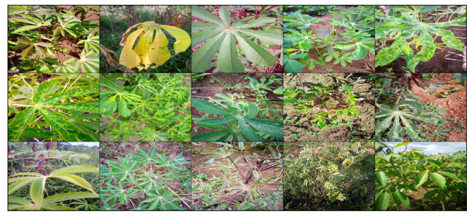
Let us picturise a few training images.

def show_example(img, label):
    print('Label: ', dataset.classes[label], "("+str(label)+")")
    plt.imshow(img.permute(1, 2, 0))

img, label = dataset[0]
show_example(img, label)

Label:  test (0)

cassava1

batch_size=15
data_loader = DataLoader(dataset, batch_size, shuffle=True, num_workers=4, pin_memory=True)

for images, _ in data_loader:
    print('images.shape:', images.shape)
    fig, ax = plt.subplots(figsize=(12, 12))
    ax.set_xticks([]); ax.set_yticks([])
    #denorm_images = denormalize(images, *stats)
    ax.imshow(make_grid(images, nrow=5).permute(1, 2, 0).clamp(0,1))
    break

images.shape: torch.Size([15, 3, 600, 800])

cassava2

Prepare dataset for training

In-order to avoid overfitting, we apply the following transformations while loading images from training dataset:

randomised data augmentaton: applying randomly chosen transformations such as cropping, horizondal flipping, changing brightness/contrast/saturation of images.
data normalization: to prevent the values from any one channel from disproportionately affecting the losses and gradients while training by having a higher or wider range of values than others.
Early stopping of model’s training, when validation loss starts to increase.

# Data transforms (normalization & data augmentation)

stats=((0.43043306, 0.4969931 , 0.3137205 ), (0.21940342, 0.22414596, 0.20117915))

train_tfms = tt.Compose([tt.RandomCrop((128,128), padding=4, padding_mode='reflect'), 
                         tt.RandomHorizontalFlip(), 
                         #tt.RandomRotation,
                         #tt.RandomResizedCrop(256, scale=(0.5,0.9), ratio=(1.0, 1.0)), 
                         tt.ColorJitter(brightness=0.1, contrast=0.1, saturation=0.1, hue=0.1),
                         tt.ToTensor(), 
                         tt.Normalize(*stats,inplace=True)])
valid_tfms = tt.Compose([tt.CenterCrop(128),tt.ToTensor(), tt.Normalize(*stats)])

# PyTorch datasets
train_ds = ImageFolder('./cassava-leaf-disease-image-folders-600x800/train', train_tfms)
valid_ds = ImageFolder('./cassava-leaf-disease-image-folders-600x800/test', valid_tfms)

Define data loaders for training and validation, to load the data in batches.

batch_size=10

# PyTorch data loaders
train_dl = DataLoader(train_ds, batch_size, shuffle=True, num_workers=3, pin_memory=True)
valid_dl = DataLoader(valid_ds, batch_size*2, num_workers=3, pin_memory=True)

Base Model Class and Training on GPU

Base model class

Let’s create a base model class, which contains everything except the model architecture i.e. it wil not contain the init and forward methods. We will later extend this class to try out different architectures.

def accuracy(outputs, labels):
    _, preds = torch.max(outputs, dim=1)
    return torch.tensor(torch.sum(preds == labels).item() / len(preds))

class ImageClassificationBase(nn.Module):
    def training_step(self, batch):
        images, labels = batch 
        out = self(images)                  # Generate predictions
        loss = F.cross_entropy(out, labels) # Calculate loss
        return loss
    
    def validation_step(self, batch):
        images, labels = batch 
        out = self(images)                    # Generate predictions
        loss = F.cross_entropy(out, labels)   # Calculate loss
        acc = accuracy(out, labels)           # Calculate accuracy
        return {'val_loss': loss.detach(), 'val_acc': acc}
        
    def validation_epoch_end(self, outputs):
        batch_losses = [x['val_loss'] for x in outputs]
        epoch_loss = torch.stack(batch_losses).mean()   # Combine losses
        batch_accs = [x['val_acc'] for x in outputs]
        epoch_acc = torch.stack(batch_accs).mean()      # Combine accuracies
        return {'val_loss': epoch_loss.item(), 'val_acc': epoch_acc.item()}
    
    def epoch_end(self, epoch, result):
        print("Epoch [{}], last_lr: {:.5f}, train_loss: {:.4f}, val_loss: {:.4f}, val_acc: {:.4f}".format(
            epoch, result['lrs'][-1], result['train_loss'], result['val_loss'], result['val_acc']))

Using GPU

To seamlessly use a GPU, if one is available, we define a couple of helper functions (get_default_device & to_device) and a helper class DeviceDataLoader to move our model & data to the GPU as required.

def get_default_device():
    """Pick GPU if available, else CPU"""
    if torch.cuda.is_available():
        return torch.device('cuda')
    else:
        return torch.device('cpu')
    
def to_device(data, device):
    """Move tensor(s) to chosen device"""
    if isinstance(data, (list,tuple)):
        return [to_device(x, device) for x in data]
    return data.to(device, non_blocking=True)

class DeviceDataLoader():
    """Wrap a dataloader to move data to a device"""
    def __init__(self, dl, device):
        self.dl = dl
        self.device = device
        
    def __iter__(self):
        """Yield a batch of data after moving it to device"""
        for b in self.dl: 
            yield to_device(b, self.device)

    def __len__(self):
        """Number of batches"""
        return len(self.dl)

device = get_default_device()
device

device(type='cuda')

Let’s move our data loaders to the appropriate device.

train_dl = DeviceDataLoader(train_dl, device)
valid_dl = DeviceDataLoader(valid_dl, device)

Helper functions for plotting loss and accuracy

Let us also define a couple of helper functions for plotting the losses & accuracies.

def plot_losses(history):
    train_losses = [x.get('train_loss') for x in history]
    val_losses = [x['val_loss'] for x in history]
    plt.plot(train_losses, '-bx')
    plt.plot(val_losses, '-rx')
    plt.xlabel('epoch')
    plt.ylabel('loss')
    plt.legend(['Training', 'Validation'])
    plt.title('Loss vs. No. of epochs');

def plot_accuracies(history):
    accuracies = [x['val_acc'] for x in history]
    plt.plot(accuracies, '-x')
    plt.xlabel('epoch')
    plt.ylabel('accuracy')
    plt.title('Accuracy vs. No. of epochs');

def plot_lrs(history):
    lrs = np.concatenate([x.get('lrs', []) for x in history])
    plt.plot(lrs)
    plt.xlabel('Batch no.')
    plt.ylabel('Learning rate')
    plt.title('Learning Rate vs. Batch no.');

Training loop

We define a fit_one_cycle function for training the model. We do the following processes in the fit_one_cycle function to improve its performance.

Learning rate scheduling: Instead of using a fixed learning rate, we will use a learning rate scheduler, which will change the learning rate after every batch of training. There are many strategies for varying the learning rate during training, and the one we’ll use is called the “One Cycle Learning Rate Policy”, which involves starting with a low learning rate, gradually increasing it batch-by-batch to a high learning rate for about 30% of epochs, then gradually decreasing it to a very low value for the remaining epochs. [Source]
Weight decay: We also use weight decay, which is yet another regularization technique which prevents the weights from becoming too large by adding an additional term to the loss function.[Source]
Gradient clipping: Apart from the layer weights and outputs, it also helpful to limit the values of gradients to a small range to prevent undesirable changes in parameters due to large gradient values. This simple yet effective technique is called gradient clipping. [Source]

Let’s define a fit_one_cycle function now. We’ll also record the learning rate used for each batch.

from tqdm.notebook import tqdm

@torch.no_grad() 
def evaluate(model, val_loader):
    model.eval() 
    outputs = [model.validation_step(batch) for batch in val_loader]
    return model.validation_epoch_end(outputs)

def get_lr(optimizer):
    for param_group in optimizer.param_groups:
        return param_group['lr']

def fit_one_cycle(epochs, max_lr, model, train_loader, val_loader, 
                  weight_decay=0, grad_clip=None, opt_func=torch.optim.SGD):
    torch.cuda.empty_cache() 
    history = [] 
    
    # Set up cutom optimizer with weight decay
    optimizer = opt_func(model.parameters(), max_lr, weight_decay=weight_decay)
    # Set up one-cycle learning rate scheduler
    sched = torch.optim.lr_scheduler.OneCycleLR(optimizer, max_lr, epochs=epochs, 
                                                steps_per_epoch=len(train_loader))
                                                  #steps_per_epoch= batches/ epoch
    for epoch in range(epochs):
        # Training Phase 
        model.train() #batchnorm layers can train their parameters beta and gamma, dropout can drop 20% of values
        train_losses = []
        lrs = []
        for batch in tqdm(train_loader):
            loss = model.training_step(batch)
            train_losses.append(loss)
            loss.backward()
            
            # Gradient clipping
            if grad_clip: #if any gradients > set value, hey get clipped
                nn.utils.clip_grad_value_(model.parameters(), grad_clip)
            
            optimizer.step() # perform gradient descent, add weight decay to loss, derivative for weight decay, perform gradient decsendt
            optimizer.zero_grad()
            
            # Record & update learning rate
            lrs.append(get_lr(optimizer)) # record lr for each batch
            sched.step() #calc next lr based on one cycle policy
        
        # Validation phase
        result = evaluate(model, val_loader)
        result['train_loss'] = torch.stack(train_losses).mean().item()
        result['lrs'] = lrs
        model.epoch_end(epoch, result)
        history.append(result)
    return history

Model-1: Feed Forward Neural Networks

input_size= 3*128*128

class FeedFwdModel(ImageClassificationBase):
    def __init__(self, input_size,output_size):
        super().__init__()
        self.linear1=nn.Linear(input_size,32)
        self.linear2=nn.Linear(32,32)
        self.linear3=nn.Linear(32,output_size)
        
    def forward(self, xb):
        # Flatten images into vectors
        out = xb.view(xb.size(0), -1)
        # Apply layers & activation functions
        out=self.linear1(out)
        out=F.relu(out)
        out=self.linear2(out)
        out=F.relu(out)
        out=self.linear3(out)
        out=F.relu(out)
        return out

You can now instantiate the model, and move it the appropriate device.

model= to_device(FeedFwdModel(input_size,len(train_ds.classes)), device)

history = [evaluate(model, valid_dl)]
history

[{'val_loss': 1.6378871202468872, 'val_acc': 0.0621495321393013}]

epochs = 8
max_lr = 0.01
grad_clip = 0.1
weight_decay = 1e-4
opt_func = torch.optim.Adam

%%time
history += fit_one_cycle(epochs, max_lr, model, train_dl, valid_dl, 
                             grad_clip=grad_clip, 
                             weight_decay=weight_decay, 
                             opt_func=opt_func)

  0%|          | 0/1927 [00:00<?, ?it/s]

Epoch [0], last_lr: 0.00396, train_loss: 1.6068, val_loss: 1.6045, val_acc: 0.0561

  0%|          | 0/1927 [00:00<?, ?it/s]

Epoch [1], last_lr: 0.00936, train_loss: 1.6418, val_loss: 2.7624, val_acc: 0.0654

  0%|          | 0/1927 [00:00<?, ?it/s]

Epoch [2], last_lr: 0.00972, train_loss: 1.6118, val_loss: 1.6094, val_acc: 0.0505

  0%|          | 0/1927 [00:00<?, ?it/s]

Epoch [3], last_lr: 0.00812, train_loss: 1.7070, val_loss: 1.6094, val_acc: 0.0505

  0%|          | 0/1927 [00:00<?, ?it/s]

Epoch [4], last_lr: 0.00556, train_loss: 1.6094, val_loss: 1.6094, val_acc: 0.0505

  0%|          | 0/1927 [00:00<?, ?it/s]

Epoch [5], last_lr: 0.00283, train_loss: 1.6338, val_loss: 1.6094, val_acc: 0.0505

  0%|          | 0/1927 [00:00<?, ?it/s]

Epoch [6], last_lr: 0.00077, train_loss: 1.6094, val_loss: 1.6094, val_acc: 0.0505

  0%|          | 0/1927 [00:00<?, ?it/s]

Epoch [7], last_lr: 0.00000, train_loss: 1.6094, val_loss: 1.6094, val_acc: 0.0505
CPU times: user 1min 39s, sys: 19.8 s, total: 1min 59s
Wall time: 29min 1s

train_time='29:01'

plot_accuracies(history)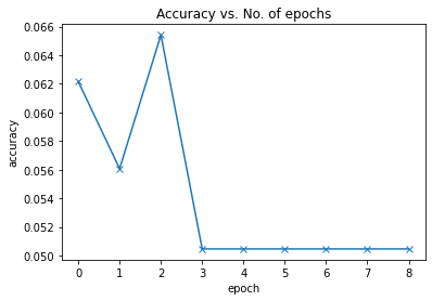

cassava3

plot_losses(history)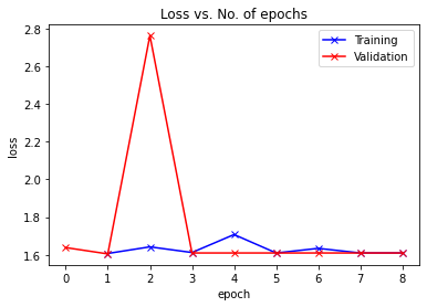

cassava4

plot_lrs(history)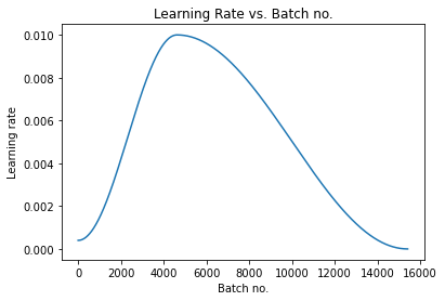

cassava5

Let us record the hyperparameters and final metrics achieved by the model for reference, analysis and comparison. We can record them using jovian.log_hyperparams.

jovian.reset()
jovian.log_hyperparams(arch='feed forward network', 
                       epochs=epochs, 
                       lr=max_lr, 
                       scheduler='one-cycle', 
                       weight_decay=weight_decay, 
                       grad_clip=grad_clip,
                       opt=opt_func.__name__)

[jovian] Hyperparams logged.[0m

jovian.log_metrics(val_loss=history[-1]['val_loss'], 
                   val_acc=history[-1]['val_acc'],
                   train_loss=history[-1]['train_loss'],
                   time=train_time)

[jovian] Metrics logged.[0m

torch.save(model.state_dict(), 'cassava-feedfwd.pth')

jovian.commit(project='cassava_project', environment=None, outputs=['cassava-feedfwd.pth'])

<IPython.core.display.Javascript object>

[jovian] Attempting to save notebook..[0m
[jovian] Detected Kaggle notebook...[0m
[jovian] Uploading notebook to https://jovian.ai/aswiniabraham/cassava_project[0m

<IPython.core.display.Javascript object>

Model-2: Convolutional Neural Networks

class CnnModel(ImageClassificationBase):
    def __init__(self, num_classes):
        super().__init__()
        self.network = nn.Sequential(
            nn.Conv2d(3, 32, kernel_size=3, padding=1),
            nn.ReLU(),
            nn.Conv2d(32, 64, kernel_size=3, stride=1, padding=1),
            nn.ReLU(),
            nn.MaxPool2d(2, 2), # output: 64 x 64 x 64

            nn.Conv2d(64, 128, kernel_size=3, stride=1, padding=1),
            nn.ReLU(),
            nn.Conv2d(128, 128, kernel_size=3, stride=1, padding=1),
            nn.ReLU(),
            nn.MaxPool2d(2, 2), # output: 128 x 32 x 32

            nn.Conv2d(128, 256, kernel_size=3, stride=1, padding=1),
            nn.ReLU(),
            nn.Conv2d(256, 256, kernel_size=3, stride=1, padding=1),
            nn.ReLU(),
            nn.MaxPool2d(2, 2), # output: 256 x 16 x 16

            nn.Flatten(), 
            nn.Linear(256*16*16, 4096),
            nn.ReLU(),
            nn.Linear(4096, 256),
            nn.ReLU(),
            nn.Linear(256, num_classes))
        
    def forward(self, xb):
        return self.network(xb)

model= CnnModel(len(train_ds.classes))
to_device(model, device)

CnnModel(
  (network): Sequential(
    (0): Conv2d(3, 32, kernel_size=(3, 3), stride=(1, 1), padding=(1, 1))
    (1): ReLU()
    (2): Conv2d(32, 64, kernel_size=(3, 3), stride=(1, 1), padding=(1, 1))
    (3): ReLU()
    (4): MaxPool2d(kernel_size=2, stride=2, padding=0, dilation=1, ceil_mode=False)
    (5): Conv2d(64, 128, kernel_size=(3, 3), stride=(1, 1), padding=(1, 1))
    (6): ReLU()
    (7): Conv2d(128, 128, kernel_size=(3, 3), stride=(1, 1), padding=(1, 1))
    (8): ReLU()
    (9): MaxPool2d(kernel_size=2, stride=2, padding=0, dilation=1, ceil_mode=False)
    (10): Conv2d(128, 256, kernel_size=(3, 3), stride=(1, 1), padding=(1, 1))
    (11): ReLU()
    (12): Conv2d(256, 256, kernel_size=(3, 3), stride=(1, 1), padding=(1, 1))
    (13): ReLU()
    (14): MaxPool2d(kernel_size=2, stride=2, padding=0, dilation=1, ceil_mode=False)
    (15): Flatten(start_dim=1, end_dim=-1)
    (16): Linear(in_features=65536, out_features=4096, bias=True)
    (17): ReLU()
    (18): Linear(in_features=4096, out_features=256, bias=True)
    (19): ReLU()
    (20): Linear(in_features=256, out_features=5, bias=True)
  )
)

history= []

history = [evaluate(model, valid_dl)]
history

[{'val_loss': 1.5846003293991089, 'val_acc': 0.10794392973184586}]

epochs = 8
max_lr = 0.01
grad_clip = 0.1
weight_decay = 1e-4
opt_func = torch.optim.Adam

%%time
history += fit_one_cycle(epochs, max_lr, model, train_dl, valid_dl, 
                             grad_clip=grad_clip, 
                             weight_decay=weight_decay, 
                             opt_func=opt_func)

  0%|          | 0/1927 [00:00<?, ?it/s]

Epoch [0], last_lr: 0.00396, train_loss: 1.1939, val_loss: 1.1860, val_acc: 0.6145

  0%|          | 0/1927 [00:00<?, ?it/s]

Epoch [1], last_lr: 0.00936, train_loss: 34.7533, val_loss: 1.1943, val_acc: 0.6145

  0%|          | 0/1927 [00:00<?, ?it/s]

Epoch [2], last_lr: 0.00972, train_loss: 16609.8730, val_loss: 1.1914, val_acc: 0.6145

  0%|          | 0/1927 [00:00<?, ?it/s]

Epoch [3], last_lr: 0.00812, train_loss: 4.8816, val_loss: 1.1838, val_acc: 0.6145

  0%|          | 0/1927 [00:00<?, ?it/s]

Epoch [4], last_lr: 0.00556, train_loss: 1.1995, val_loss: 1.1841, val_acc: 0.6145

  0%|          | 0/1927 [00:00<?, ?it/s]

Epoch [5], last_lr: 0.00283, train_loss: 1.1852, val_loss: 1.1838, val_acc: 0.6145

  0%|          | 0/1927 [00:00<?, ?it/s]

Epoch [6], last_lr: 0.00077, train_loss: 1.1833, val_loss: 1.1839, val_acc: 0.6145

  0%|          | 0/1927 [00:00<?, ?it/s]

Epoch [7], last_lr: 0.00000, train_loss: 1.1834, val_loss: 1.1837, val_acc: 0.6145
CPU times: user 3min 30s, sys: 21.7 s, total: 3min 51s
Wall time: 30min 46s

train_time='30:46'

plot_accuracies(history)

m2_1

plot_losses(history)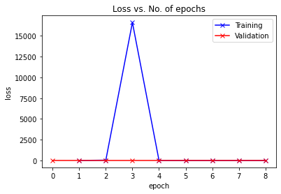

m2_2

Let us record the hyperparameters and final metrics achieved by the model.

jovian.reset()
jovian.log_hyperparams(arch='convolutional neural network', 
                       epochs=epochs, 
                       lr=max_lr, 
                       scheduler='one-cycle', 
                       weight_decay=weight_decay, 
                       grad_clip=grad_clip,
                       opt=opt_func.__name__)

[jovian] Hyperparams logged.[0m

jovian.log_metrics(val_loss=history[-1]['val_loss'], 
                   val_acc=history[-1]['val_acc'],
                   train_loss=history[-1]['train_loss'],
                   time=train_time)

[jovian] Metrics logged.[0m

torch.save(model.state_dict(), 'cnn.pth')

jovian.commit(project='cassava_project', environment=None, outputs=['cnn.pth'])

<IPython.core.display.Javascript object>

[jovian] Attempting to save notebook..[0m
[jovian] Detected Kaggle notebook...[0m
[jovian] Uploading notebook to https://jovian.ai/aswiniabraham/cassava_project[0m

<IPython.core.display.Javascript object>

Model-3: Resnet34 and transfer learning

# Data transforms (normalization & data augmentation)

imagenet_stats = ([0.485, 0.456, 0.406], [0.229, 0.224, 0.225])
train_tfms = tt.Compose([tt.RandomCrop((128,128), padding=4, padding_mode='reflect'), 
                         tt.RandomHorizontalFlip(), 
                         #tt.RandomRotation,
                         #tt.RandomResizedCrop(256, scale=(0.5,0.9), ratio=(1.0, 1.0)), 
                         tt.ColorJitter(brightness=0.1, contrast=0.1, saturation=0.1, hue=0.1),
                         tt.ToTensor(), 
                         tt.Normalize(*imagenet_stats,inplace=True)])
valid_tfms = tt.Compose([tt.CenterCrop(128),tt.ToTensor(), tt.Normalize(*imagenet_stats)])

# PyTorch datasets
train_ds = ImageFolder('./cassava-leaf-disease-image-folders-600x800/train', train_tfms)
valid_ds = ImageFolder('./cassava-leaf-disease-image-folders-600x800/test', valid_tfms)

batch_size=10

# PyTorch data loaders
train_dl = DataLoader(train_ds, batch_size, shuffle=True, num_workers=3, pin_memory=True)
valid_dl = DataLoader(valid_ds, batch_size*2, num_workers=3, pin_memory=True)

train_dl = DeviceDataLoader(train_dl, device)
valid_dl = DeviceDataLoader(valid_dl, device)

from torchvision import models

class Resnet34Model(ImageClassificationBase):
    def __init__(self, num_classes, pretrained=True):
        super().__init__()
        # Use a pretrained model
        self.network = models.resnet34(pretrained=pretrained)
        # Replace last layer
        self.network.fc = nn.Linear(self.network.fc.in_features, num_classes)

    def forward(self, xb):
        return self.network(xb)

model = to_device(Resnet34Model(len(train_ds.classes)), device)

history= []

history = [evaluate(model, valid_dl)]
history

[{'val_loss': 1.6652694940567017, 'val_acc': 0.24976633489131927}]

epochs = 8
max_lr = 0.01
grad_clip = 0.1
weight_decay = 1e-4
opt_func = torch.optim.Adam

%%time
history += fit_one_cycle(epochs, max_lr, model, train_dl, valid_dl, 
                             grad_clip=grad_clip, 
                             weight_decay=weight_decay, 
                             opt_func=opt_func)

  0%|          | 0/1927 [00:00<?, ?it/s]

Epoch [0], last_lr: 0.00396, train_loss: 1.2018, val_loss: 1.7423, val_acc: 0.6206

  0%|          | 0/1927 [00:00<?, ?it/s]

Epoch [1], last_lr: 0.00936, train_loss: 1.1898, val_loss: 1.2172, val_acc: 0.5972

  0%|          | 0/1927 [00:00<?, ?it/s]

Epoch [2], last_lr: 0.00972, train_loss: 1.1844, val_loss: 1.1469, val_acc: 0.6196

  0%|          | 0/1927 [00:00<?, ?it/s]

Epoch [3], last_lr: 0.00812, train_loss: 1.1836, val_loss: 1.1837, val_acc: 0.6145

  0%|          | 0/1927 [00:00<?, ?it/s]

Epoch [4], last_lr: 0.00556, train_loss: 1.1753, val_loss: 1.0930, val_acc: 0.6248

  0%|          | 0/1927 [00:00<?, ?it/s]

Epoch [5], last_lr: 0.00283, train_loss: 1.1428, val_loss: 1.0670, val_acc: 0.6224

  0%|          | 0/1927 [00:00<?, ?it/s]

Epoch [6], last_lr: 0.00077, train_loss: 1.1171, val_loss: 1.0275, val_acc: 0.6290

  0%|          | 0/1927 [00:00<?, ?it/s]

Epoch [7], last_lr: 0.00000, train_loss: 1.0956, val_loss: 0.9982, val_acc: 0.6352
CPU times: user 16min 30s, sys: 30.2 s, total: 17min
Wall time: 38min 46s

train_time='38:46'

plot_accuracies(history)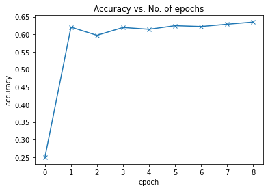

m3_1

plot_losses(history)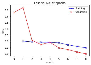

m3_2

Let us record the hyperparameters and final metrics achieved by the model.

jovian.reset()
jovian.log_hyperparams(arch='Resnet34 network', 
                       epochs=epochs, 
                       lr=max_lr, 
                       scheduler='one-cycle', 
                       weight_decay=weight_decay, 
                       grad_clip=grad_clip,
                       opt=opt_func.__name__)

[jovian] Hyperparams logged.[0m

jovian.log_metrics(val_loss=history[-1]['val_loss'], 
                   val_acc=history[-1]['val_acc'],
                   train_loss=history[-1]['train_loss'],
                   time=train_time)

[jovian] Metrics logged.[0m

torch.save(model.state_dict(), 'cassava-resnet34.pth')

jovian.commit(project='cassava_project', environment=None, outputs=['cassava-resnet34.pth'])

<IPython.core.display.Javascript object>

[jovian] Attempting to save notebook..[0m
[jovian] Detected Kaggle notebook...[0m
[jovian] Uploading notebook to https://jovian.ai/aswiniabraham/cassava_project[0m

<IPython.core.display.Javascript object>

Model-4: EfficientNet B4 model

# Data transforms (normalization & data augmentation)

imagenet_stats = ([0.485, 0.456, 0.406], [0.229, 0.224, 0.225])
train_tfms = tt.Compose([tt.RandomCrop((128,128), padding=4, padding_mode='reflect'), 
                         tt.RandomHorizontalFlip(), 
                         #tt.RandomRotation,
                         #tt.RandomResizedCrop(256, scale=(0.5,0.9), ratio=(1.0, 1.0)), 
                         tt.ColorJitter(brightness=0.1, contrast=0.1, saturation=0.1, hue=0.1),
                         tt.ToTensor(), 
                         tt.Normalize(*imagenet_stats,inplace=True)])
valid_tfms = tt.Compose([tt.CenterCrop(128),tt.ToTensor(), tt.Normalize(*imagenet_stats)])

# PyTorch datasets
train_ds = ImageFolder('./cassava-leaf-disease-image-folders-600x800/train', train_tfms)
valid_ds = ImageFolder('./cassava-leaf-disease-image-folders-600x800/test', valid_tfms)

batch_size=10

# PyTorch data loaders
train_dl = DataLoader(train_ds, batch_size, shuffle=True, num_workers=3, pin_memory=True)
valid_dl = DataLoader(valid_ds, batch_size*2, num_workers=3, pin_memory=True)

train_dl = DeviceDataLoader(train_dl, device)
valid_dl = DeviceDataLoader(valid_dl, device)

! pip install efficientnet-pytorch

from efficientnet_pytorch import EfficientNet

class Enetb4Model(ImageClassificationBase):
    def __init__(self, num_classes, pretrained=True):
        super().__init__()
        # Use a pretrained model
        self.network = EfficientNet.from_pretrained('efficientnet-b4', num_classes=num_classes)

    def forward(self, xb):
        return self.network(xb)

model = to_device(Enetb4Model(len(train_ds.classes)), device)

history= []

history = [evaluate(model, valid_dl)]
history

epochs = 8
max_lr = 0.01
grad_clip = 0.1
weight_decay = 1e-4
opt_func = torch.optim.Adam

%%time
history += fit_one_cycle(epochs, max_lr, model, train_dl, valid_dl, 
                             grad_clip=grad_clip, 
                             weight_decay=weight_decay, 
                             opt_func=opt_func)

train_time='1:05:57'

plot_accuracies(history)

plot_losses(history)

Let us record the hyperparameters and final metrics achieved by the model.

!pip install jovian --upgrade --quiet

import jovian

jovian.reset()
jovian.log_hyperparams(arch='Effiecientnet B4', 
                       epochs=epochs, 
                       lr=max_lr, 
                       scheduler='one-cycle', 
                       weight_decay=weight_decay, 
                       grad_clip=grad_clip,
                       opt=opt_func.__name__)

jovian.log_metrics(val_loss=history[-1]['val_loss'], 
                   val_acc=history[-1]['val_acc'],
                   train_loss=history[-1]['train_loss'],
                   time=train_time)

torch.save(model.state_dict(), 'cassava-enetb4.pth')

jovian.commit(project='cassava_project', environment=None, outputs=['cassava-enetb4.pth'])

os.getcwd()

os.listdir('./')

from IPython.display import FileLink
FileLink(r'cassava-enetb4.pth')

Model-5: Resnext50_32x4d

# ================================================
# resnext50_32x4d architecture
# ================================================

from torchvision import models

class ResnextModel(ImageClassificationBase):
    def __init__(self, num_classes, pretrained=True):
        super().__init__()
        # Use a pretrained model
        self.network = models.resnext50_32x4d(pretrained=pretrained)
        # Replace last layer
        self.network.fc = nn.Linear(self.network.fc.in_features, num_classes)

    def forward(self, xb):
        return self.network(xb)

model = ResnextModel(len(train_ds.classes), pretrained= True)

to_device(model, device)

ResnextModel(
  (network): ResNet(
    (conv1): Conv2d(3, 64, kernel_size=(7, 7), stride=(2, 2), padding=(3, 3), bias=False)
    (bn1): BatchNorm2d(64, eps=1e-05, momentum=0.1, affine=True, track_running_stats=True)
    (relu): ReLU(inplace=True)
    (maxpool): MaxPool2d(kernel_size=3, stride=2, padding=1, dilation=1, ceil_mode=False)
    (layer1): Sequential(
      (0): Bottleneck(
        (conv1): Conv2d(64, 128, kernel_size=(1, 1), stride=(1, 1), bias=False)
        (bn1): BatchNorm2d(128, eps=1e-05, momentum=0.1, affine=True, track_running_stats=True)
        (conv2): Conv2d(128, 128, kernel_size=(3, 3), stride=(1, 1), padding=(1, 1), groups=32, bias=False)
        (bn2): BatchNorm2d(128, eps=1e-05, momentum=0.1, affine=True, track_running_stats=True)
        (conv3): Conv2d(128, 256, kernel_size=(1, 1), stride=(1, 1), bias=False)
        (bn3): BatchNorm2d(256, eps=1e-05, momentum=0.1, affine=True, track_running_stats=True)
        (relu): ReLU(inplace=True)
        (downsample): Sequential(
          (0): Conv2d(64, 256, kernel_size=(1, 1), stride=(1, 1), bias=False)
          (1): BatchNorm2d(256, eps=1e-05, momentum=0.1, affine=True, track_running_stats=True)
        )
      )
      (1): Bottleneck(
        (conv1): Conv2d(256, 128, kernel_size=(1, 1), stride=(1, 1), bias=False)
        (bn1): BatchNorm2d(128, eps=1e-05, momentum=0.1, affine=True, track_running_stats=True)
        (conv2): Conv2d(128, 128, kernel_size=(3, 3), stride=(1, 1), padding=(1, 1), groups=32, bias=False)
        (bn2): BatchNorm2d(128, eps=1e-05, momentum=0.1, affine=True, track_running_stats=True)
        (conv3): Conv2d(128, 256, kernel_size=(1, 1), stride=(1, 1), bias=False)
        (bn3): BatchNorm2d(256, eps=1e-05, momentum=0.1, affine=True, track_running_stats=True)
        (relu): ReLU(inplace=True)
      )
      (2): Bottleneck(
        (conv1): Conv2d(256, 128, kernel_size=(1, 1), stride=(1, 1), bias=False)
        (bn1): BatchNorm2d(128, eps=1e-05, momentum=0.1, affine=True, track_running_stats=True)
        (conv2): Conv2d(128, 128, kernel_size=(3, 3), stride=(1, 1), padding=(1, 1), groups=32, bias=False)
        (bn2): BatchNorm2d(128, eps=1e-05, momentum=0.1, affine=True, track_running_stats=True)
        (conv3): Conv2d(128, 256, kernel_size=(1, 1), stride=(1, 1), bias=False)
        (bn3): BatchNorm2d(256, eps=1e-05, momentum=0.1, affine=True, track_running_stats=True)
        (relu): ReLU(inplace=True)
      )
    )
    (layer2): Sequential(
      (0): Bottleneck(
        (conv1): Conv2d(256, 256, kernel_size=(1, 1), stride=(1, 1), bias=False)
        (bn1): BatchNorm2d(256, eps=1e-05, momentum=0.1, affine=True, track_running_stats=True)
        (conv2): Conv2d(256, 256, kernel_size=(3, 3), stride=(2, 2), padding=(1, 1), groups=32, bias=False)
        (bn2): BatchNorm2d(256, eps=1e-05, momentum=0.1, affine=True, track_running_stats=True)
        (conv3): Conv2d(256, 512, kernel_size=(1, 1), stride=(1, 1), bias=False)
        (bn3): BatchNorm2d(512, eps=1e-05, momentum=0.1, affine=True, track_running_stats=True)
        (relu): ReLU(inplace=True)
        (downsample): Sequential(
          (0): Conv2d(256, 512, kernel_size=(1, 1), stride=(2, 2), bias=False)
          (1): BatchNorm2d(512, eps=1e-05, momentum=0.1, affine=True, track_running_stats=True)
        )
      )
      (1): Bottleneck(
        (conv1): Conv2d(512, 256, kernel_size=(1, 1), stride=(1, 1), bias=False)
        (bn1): BatchNorm2d(256, eps=1e-05, momentum=0.1, affine=True, track_running_stats=True)
        (conv2): Conv2d(256, 256, kernel_size=(3, 3), stride=(1, 1), padding=(1, 1), groups=32, bias=False)
        (bn2): BatchNorm2d(256, eps=1e-05, momentum=0.1, affine=True, track_running_stats=True)
        (conv3): Conv2d(256, 512, kernel_size=(1, 1), stride=(1, 1), bias=False)
        (bn3): BatchNorm2d(512, eps=1e-05, momentum=0.1, affine=True, track_running_stats=True)
        (relu): ReLU(inplace=True)
      )
      (2): Bottleneck(
        (conv1): Conv2d(512, 256, kernel_size=(1, 1), stride=(1, 1), bias=False)
        (bn1): BatchNorm2d(256, eps=1e-05, momentum=0.1, affine=True, track_running_stats=True)
        (conv2): Conv2d(256, 256, kernel_size=(3, 3), stride=(1, 1), padding=(1, 1), groups=32, bias=False)
        (bn2): BatchNorm2d(256, eps=1e-05, momentum=0.1, affine=True, track_running_stats=True)
        (conv3): Conv2d(256, 512, kernel_size=(1, 1), stride=(1, 1), bias=False)
        (bn3): BatchNorm2d(512, eps=1e-05, momentum=0.1, affine=True, track_running_stats=True)
        (relu): ReLU(inplace=True)
      )
      (3): Bottleneck(
        (conv1): Conv2d(512, 256, kernel_size=(1, 1), stride=(1, 1), bias=False)
        (bn1): BatchNorm2d(256, eps=1e-05, momentum=0.1, affine=True, track_running_stats=True)
        (conv2): Conv2d(256, 256, kernel_size=(3, 3), stride=(1, 1), padding=(1, 1), groups=32, bias=False)
        (bn2): BatchNorm2d(256, eps=1e-05, momentum=0.1, affine=True, track_running_stats=True)
        (conv3): Conv2d(256, 512, kernel_size=(1, 1), stride=(1, 1), bias=False)
        (bn3): BatchNorm2d(512, eps=1e-05, momentum=0.1, affine=True, track_running_stats=True)
        (relu): ReLU(inplace=True)
      )
    )
    (layer3): Sequential(
      (0): Bottleneck(
        (conv1): Conv2d(512, 512, kernel_size=(1, 1), stride=(1, 1), bias=False)
        (bn1): BatchNorm2d(512, eps=1e-05, momentum=0.1, affine=True, track_running_stats=True)
        (conv2): Conv2d(512, 512, kernel_size=(3, 3), stride=(2, 2), padding=(1, 1), groups=32, bias=False)
        (bn2): BatchNorm2d(512, eps=1e-05, momentum=0.1, affine=True, track_running_stats=True)
        (conv3): Conv2d(512, 1024, kernel_size=(1, 1), stride=(1, 1), bias=False)
        (bn3): BatchNorm2d(1024, eps=1e-05, momentum=0.1, affine=True, track_running_stats=True)
        (relu): ReLU(inplace=True)
        (downsample): Sequential(
          (0): Conv2d(512, 1024, kernel_size=(1, 1), stride=(2, 2), bias=False)
          (1): BatchNorm2d(1024, eps=1e-05, momentum=0.1, affine=True, track_running_stats=True)
        )
      )
      (1): Bottleneck(
        (conv1): Conv2d(1024, 512, kernel_size=(1, 1), stride=(1, 1), bias=False)
        (bn1): BatchNorm2d(512, eps=1e-05, momentum=0.1, affine=True, track_running_stats=True)
        (conv2): Conv2d(512, 512, kernel_size=(3, 3), stride=(1, 1), padding=(1, 1), groups=32, bias=False)
        (bn2): BatchNorm2d(512, eps=1e-05, momentum=0.1, affine=True, track_running_stats=True)
        (conv3): Conv2d(512, 1024, kernel_size=(1, 1), stride=(1, 1), bias=False)
        (bn3): BatchNorm2d(1024, eps=1e-05, momentum=0.1, affine=True, track_running_stats=True)
        (relu): ReLU(inplace=True)
      )
      (2): Bottleneck(
        (conv1): Conv2d(1024, 512, kernel_size=(1, 1), stride=(1, 1), bias=False)
        (bn1): BatchNorm2d(512, eps=1e-05, momentum=0.1, affine=True, track_running_stats=True)
        (conv2): Conv2d(512, 512, kernel_size=(3, 3), stride=(1, 1), padding=(1, 1), groups=32, bias=False)
        (bn2): BatchNorm2d(512, eps=1e-05, momentum=0.1, affine=True, track_running_stats=True)
        (conv3): Conv2d(512, 1024, kernel_size=(1, 1), stride=(1, 1), bias=False)
        (bn3): BatchNorm2d(1024, eps=1e-05, momentum=0.1, affine=True, track_running_stats=True)
        (relu): ReLU(inplace=True)
      )
      (3): Bottleneck(
        (conv1): Conv2d(1024, 512, kernel_size=(1, 1), stride=(1, 1), bias=False)
        (bn1): BatchNorm2d(512, eps=1e-05, momentum=0.1, affine=True, track_running_stats=True)
        (conv2): Conv2d(512, 512, kernel_size=(3, 3), stride=(1, 1), padding=(1, 1), groups=32, bias=False)
        (bn2): BatchNorm2d(512, eps=1e-05, momentum=0.1, affine=True, track_running_stats=True)
        (conv3): Conv2d(512, 1024, kernel_size=(1, 1), stride=(1, 1), bias=False)
        (bn3): BatchNorm2d(1024, eps=1e-05, momentum=0.1, affine=True, track_running_stats=True)
        (relu): ReLU(inplace=True)
      )
      (4): Bottleneck(
        (conv1): Conv2d(1024, 512, kernel_size=(1, 1), stride=(1, 1), bias=False)
        (bn1): BatchNorm2d(512, eps=1e-05, momentum=0.1, affine=True, track_running_stats=True)
        (conv2): Conv2d(512, 512, kernel_size=(3, 3), stride=(1, 1), padding=(1, 1), groups=32, bias=False)
        (bn2): BatchNorm2d(512, eps=1e-05, momentum=0.1, affine=True, track_running_stats=True)
        (conv3): Conv2d(512, 1024, kernel_size=(1, 1), stride=(1, 1), bias=False)
        (bn3): BatchNorm2d(1024, eps=1e-05, momentum=0.1, affine=True, track_running_stats=True)
        (relu): ReLU(inplace=True)
      )
      (5): Bottleneck(
        (conv1): Conv2d(1024, 512, kernel_size=(1, 1), stride=(1, 1), bias=False)
        (bn1): BatchNorm2d(512, eps=1e-05, momentum=0.1, affine=True, track_running_stats=True)
        (conv2): Conv2d(512, 512, kernel_size=(3, 3), stride=(1, 1), padding=(1, 1), groups=32, bias=False)
        (bn2): BatchNorm2d(512, eps=1e-05, momentum=0.1, affine=True, track_running_stats=True)
        (conv3): Conv2d(512, 1024, kernel_size=(1, 1), stride=(1, 1), bias=False)
        (bn3): BatchNorm2d(1024, eps=1e-05, momentum=0.1, affine=True, track_running_stats=True)
        (relu): ReLU(inplace=True)
      )
    )
    (layer4): Sequential(
      (0): Bottleneck(
        (conv1): Conv2d(1024, 1024, kernel_size=(1, 1), stride=(1, 1), bias=False)
        (bn1): BatchNorm2d(1024, eps=1e-05, momentum=0.1, affine=True, track_running_stats=True)
        (conv2): Conv2d(1024, 1024, kernel_size=(3, 3), stride=(2, 2), padding=(1, 1), groups=32, bias=False)
        (bn2): BatchNorm2d(1024, eps=1e-05, momentum=0.1, affine=True, track_running_stats=True)
        (conv3): Conv2d(1024, 2048, kernel_size=(1, 1), stride=(1, 1), bias=False)
        (bn3): BatchNorm2d(2048, eps=1e-05, momentum=0.1, affine=True, track_running_stats=True)
        (relu): ReLU(inplace=True)
        (downsample): Sequential(
          (0): Conv2d(1024, 2048, kernel_size=(1, 1), stride=(2, 2), bias=False)
          (1): BatchNorm2d(2048, eps=1e-05, momentum=0.1, affine=True, track_running_stats=True)
        )
      )
      (1): Bottleneck(
        (conv1): Conv2d(2048, 1024, kernel_size=(1, 1), stride=(1, 1), bias=False)
        (bn1): BatchNorm2d(1024, eps=1e-05, momentum=0.1, affine=True, track_running_stats=True)
        (conv2): Conv2d(1024, 1024, kernel_size=(3, 3), stride=(1, 1), padding=(1, 1), groups=32, bias=False)
        (bn2): BatchNorm2d(1024, eps=1e-05, momentum=0.1, affine=True, track_running_stats=True)
        (conv3): Conv2d(1024, 2048, kernel_size=(1, 1), stride=(1, 1), bias=False)
        (bn3): BatchNorm2d(2048, eps=1e-05, momentum=0.1, affine=True, track_running_stats=True)
        (relu): ReLU(inplace=True)
      )
      (2): Bottleneck(
        (conv1): Conv2d(2048, 1024, kernel_size=(1, 1), stride=(1, 1), bias=False)
        (bn1): BatchNorm2d(1024, eps=1e-05, momentum=0.1, affine=True, track_running_stats=True)
        (conv2): Conv2d(1024, 1024, kernel_size=(3, 3), stride=(1, 1), padding=(1, 1), groups=32, bias=False)
        (bn2): BatchNorm2d(1024, eps=1e-05, momentum=0.1, affine=True, track_running_stats=True)
        (conv3): Conv2d(1024, 2048, kernel_size=(1, 1), stride=(1, 1), bias=False)
        (bn3): BatchNorm2d(2048, eps=1e-05, momentum=0.1, affine=True, track_running_stats=True)
        (relu): ReLU(inplace=True)
      )
    )
    (avgpool): AdaptiveAvgPool2d(output_size=(1, 1))
    (fc): Linear(in_features=2048, out_features=5, bias=True)
  )
)

history= []

history = [evaluate(model, valid_dl)]
history

[{'val_loss': 1.709054946899414, 'val_acc': 0.11039718985557556}]

%%time
history += fit_one_cycle(epochs, max_lr, model, train_dl, valid_dl, 
                             grad_clip=grad_clip, 
                             weight_decay=weight_decay, 
                             opt_func=opt_func)

  0%|          | 0/1927 [00:00<?, ?it/s]

Epoch [0], last_lr: 0.00396, train_loss: 1.1113, val_loss: 1.0380, val_acc: 0.6275

  0%|          | 0/1927 [00:00<?, ?it/s]

Epoch [1], last_lr: 0.00936, train_loss: 1.1528, val_loss: 1.6740, val_acc: 0.6145

  0%|          | 0/1927 [00:00<?, ?it/s]

Epoch [2], last_lr: 0.00972, train_loss: 1.1777, val_loss: 1.2194, val_acc: 0.6145

  0%|          | 0/1927 [00:00<?, ?it/s]

Epoch [3], last_lr: 0.00812, train_loss: 1.2058, val_loss: 1.1862, val_acc: 0.6145

  0%|          | 0/1927 [00:00<?, ?it/s]

Epoch [4], last_lr: 0.00556, train_loss: 1.2107, val_loss: 1.1467, val_acc: 0.6145

  0%|          | 0/1927 [00:00<?, ?it/s]

Epoch [5], last_lr: 0.00283, train_loss: 1.1942, val_loss: 1.1059, val_acc: 0.6221

  0%|          | 0/1927 [00:00<?, ?it/s]

Epoch [6], last_lr: 0.00077, train_loss: 1.1408, val_loss: 1.0327, val_acc: 0.6341

  0%|          | 0/1927 [00:00<?, ?it/s]

Epoch [7], last_lr: 0.00000, train_loss: 1.1161, val_loss: 1.0162, val_acc: 0.6398
CPU times: user 31min 28s, sys: 33.8 s, total: 32min 2s
Wall time: 45min 17s

train_time='45:17'

plot_accuracies(history)

m5_1

plot_losses(history)

m5_2

Let us record the hyperparameters and final metrics achieved by the model.

jovian.reset()
jovian.log_hyperparams(arch='resnext50_32x4d', 
                       epochs=epochs, 
                       lr=max_lr, 
                       scheduler='one-cycle', 
                       weight_decay=weight_decay, 
                       grad_clip=grad_clip,
                       opt=opt_func.__name__)

[jovian] Hyperparams logged.[0m

jovian.log_metrics(val_loss=history[-1]['val_loss'], 
                   val_acc=history[-1]['val_acc'],
                   train_loss=history[-1]['train_loss'],
                   time=train_time)

[jovian] Metrics logged.[0m

torch.save(model.state_dict(), 'cassava-resnext50.pth')

from IPython.display import FileLink
FileLink(r'cassava-resnext50.pth')

cassava-resnext50.pth

jovian.commit(project='cassava_project', environment=None, outputs=['cassava-resnext50.pth'])

<IPython.core.display.Javascript object>

[jovian] Attempting to save notebook..[0m
[jovian] Detected Kaggle notebook...[0m
[jovian] Uploading notebook to https://jovian.ai/aswiniabraham/cassava_project[0m

<IPython.core.display.Javascript object>

Ensemble two models

! pip install efficientnet-pytorch
#! pip install timm

# ================================================
# efficientnet-b4 architecture
# ================================================

from efficientnet_pytorch import EfficientNet

#import timm

class EnetModel(ImageClassificationBase):
    def __init__(self, num_classes, pretrained=True):
        super().__init__()
        # Use a pretrained model
        self.network = EfficientNet.from_pretrained('efficientnet-b4', num_classes=num_classes)
        #self.network=timm.create_model('tf_efficientnet_b4_ns', pretrained=pretrained)
        # Replace last layer
        #self.network.fc = nn.Linear(self.network.fc.in_features, num_classes)
    
    def forward(self, xb):
        return self.network(xb)

# ================================================
# resnext50_32x4d architecture
# ================================================

from torchvision import models

class ResnextModel(ImageClassificationBase):
    def __init__(self, num_classes, pretrained=True):
        super().__init__()
        # Use a pretrained model
        self.network = models.resnext50_32x4d(pretrained=pretrained)
        # Replace last layer
        self.network.fc = nn.Linear(self.network.fc.in_features, num_classes)

    def forward(self, xb):
        return self.network(xb)

EfficientNet.from_pretrained('efficientnet-b4', num_classes=num_classes)

models.resnext50_32x4d(pretrained=False)

# Ensemble two models

class MyEnsemble(ImageClassificationBase):
    def __init__(self, modelA, modelB, num_classes):
        super(MyEnsemble, self).__init__()
        self.modelA = modelA
        self.modelB = modelB
        # Remove last linear layer
        self.modelA.fc= nn.Identity()
        self.modelB.fc= nn.Identity()

        # Create new classifier
        self.classifier= nn.Linear(1792+2040, num_classes)
        
    def forward(self, x):
      x1= self.modelA(x.clone())
      x1= x1.view(x1.size(0),-1)
      x2= self.modelB(x)
      x2= x2.view(x2.size(0),-1)
      x= torch.cat((x1,x2),dim=1)

      x= self.classifier(F.relu(x))
      return x

MyEnsemble(modelA, modelB, len(train_ds.classes))

# Load models
modelA = EnetModel(len(train_ds.classes), pretrained= False)
modelB = ResnextModel(len(train_ds.classes), pretrained= False)

# Load state dicts
modelA.load_state_dict(torch.load('cassava-efficientnet-04_67pct_8epch.pth'))
modelB.load_state_dict(torch.load('cassava-resnext50_32x4d.pth'))

model = MyEnsemble(modelA, modelB, len(train_ds.classes))

# Load to device 
model= to_device(model, device)

epochs = 8
max_lr = 0.01
grad_clip = 0.1
weight_decay = 1e-4
opt_func = torch.optim.Adam

history = [evaluate(model, valid_dl)]
history

%%time
history += fit_one_cycle(epochs, max_lr, model, train_dl, valid_dl, 
                             grad_clip=grad_clip, 
                             weight_decay=weight_decay, 
                             opt_func=opt_func)

train_time=':'

plot_accuracies(history)

plot_losses(history)

plot_lrs(history)

Testing with individual images

def predict_image(img, model):
    # Convert to a batch of 1
    xb = to_device(img.unsqueeze(0), device)
    # Get predictions from model
    yb = model(xb)
    # Pick index with highest probability
    _, preds  = torch.max(yb, dim=1)
    # Retrieve the class label
    return train_ds.classes[preds[0].item()]

img, label = valid_ds[0]
plt.imshow(img.permute(1, 2, 0).clamp(0, 1))
print('Label:', train_ds.classes[label], ', Predicted:', predict_image(img, model))

img, label = valid_ds[1002]
plt.imshow(img.permute(1, 2, 0))
print('Label:', valid_ds.classes[label], ', Predicted:', predict_image(img, model))

img, label = valid_ds[153]
plt.imshow(img.permute(1, 2, 0))
print('Label:', train_ds.classes[label], ', Predicted:', predict_image(img, model))

Summary of training results

The table below gives the validation loss, validation accuracy and time taken for training different models for the following hyperparameters: epochs = 8 max_lr = 0.01 grad_clip = 0.1 weight_decay = 1e-4 opt_func = torch.optim.Adam

Model	val_accuracy	val_loss	time
Feed Forward Neural Network	05.05%	1.60944	29:01
Convolutional Neural Network	61.45%	1.18407	46:52
Resnet34	64.92%	0.94607	34:30
Efficientnet-B4	65.25%	0.89396	1:05:57
Resnext50_32x4d	63.98%	1.01616	45:17

Save

jovian.commit(project='cassava_project', environment=None)

<IPython.core.display.Javascript object>

[jovian] Attempting to save notebook..[0m
[jovian] Detected Kaggle notebook...[0m
[jovian] Uploading notebook to https://jovian.ai/aswiniabraham/cassava_project[0m

<IPython.core.display.Javascript object>

-->