How to Model Stock Price
1. Why do we need to model stock price?
Occasionaly, assets gets mispriced in the market – either overvalued or undervalued – for a brief period of time. Market action would eventually correct the situation, moving price back to its fair market value. To an arbitrageur, temporarily mispriced securities represent a short-term opportunity to profit, virtually without risk. A model that estimates the fair market price of a stock helps an arbitrageur to purchase the stock when they are priced lower than their fair price and sell later at a profit. Such a model is based on Arbitrage Pricing Theory (APT) that holds that an asset’s returns can be forecasted with the linear relationship of an asset’s expected returns and the macroeconomic factors that affect the asset’s risk. The expected return is the profit or loss an investor anticipates on an investment, usually expressed in percentage.
2. What factors affect the stock price?
Several studies have been conducted on factors that could affect stock returns. There are various factors that affect the stock price and they vary for the stock depending on factors like industry, technology involved etc. In this article, let us look at the factors that affect the stock price of Microsoft. The following factors have been identified to have a potential impact on Microsoft stock price:
Table1:Factors affecting stock price and their potential impact
| Factor | Impact on stock price |
|---|---|
| S&P500 index | Positive |
| Inflation | Negative |
| Industrial production | Positive |
| Term spread | Positive |
| Consumer credit | Positive |
| Credit spread | Negative |
| Money supply | Positive |
- S&P 500 is a stock market index that measures the stock performance of 500 large companies listed on stock exchanges in the United States. Many consider it to be one of the best representations of the U.S. stock market.
- Inflation is the rate at which the average price level of a basket of selected goods and services in an economy increases over some period of time. It is calculated from the Consumer Price Index (CPI) and is often expressed as a percentage. If the inflation rate increases, the return from the stock looks less attractive.
- Industrial Production is measured in terms of Industrial Production Index (IPI), a monthly economic indicator measuring real output in the manufacturing, mining, electric and gas industries, relative to a base year. A increased IPI indicate increased industrial activity and is expected to have a positive impact on the return of stocks.
- Term spread measures the difference between the interest rates of two bonds with different maturities or expiration dates. Yield spreads between Treasury bonds of different maturities indicate how investors are viewing economic conditions. Widening spreads indicates stable economic conditions in the future whereas falling spreads indicates worsening economy.
- Consumer credit is the personal debt taken to purchase goods and services. A credit card is one form of consumer credit. Although any type of personal loan could be labelled consumer credit, the term is usually used to describe unsecured debt that is taken on to buy everyday goods and services. Increased consumer credit indicate increased consumer spending, leading to increased production and transactions in the market. Hence, it has a positive impact on the stock returns.
- Credit spread measures the difference in yield between U.S. Treasury bonds and other debt securities of lesser quality, such as corporate bonds. Credit spreads widen when U.S. Treasury markets are favored over corporate bonds, typically in times of uncertainty or when economic conditions are expected to deteriorate.
- Money supply is all the currency and other liquid instruments in a country’s economy on the date measured that can be used almost as easily as cash. The more the money supply, the higher price of stock.
3. How can we model the stock return?
The total return for a stock is the sum of capital gains/losses and dividend income. To model the stock return, we first gather the input data and apply data transformations. With the transformed data, we use a linear regression model to explain the relationship between the predictors and the stock return.
3.1 Data gathering
To prepare for analysis and model development, the following data for the period March 1986 to June 2020 were collected and cleaned:
Table2:Data sources
| Data | Variable | Source |
|---|---|---|
| Microsoft stock return | MICROSOFT | finance.yahoo.com |
| S&P 500 index | SANDP | finance.yahoo.com |
| Consumer Price Index | CPI | US Inflation Calculator |
| Industrial Production Index | INDPRO | Fred Economic Data |
| Treasury bill yields | USTB3M, USTB10Y | Fred Economic Data |
| Consumer Credit | CCREDIT | Fred Economic Data |
| Credit Spread | BMINUSA | Fred Economic Data |
| Money Supply | M1SUPPLY | Fred Economic Data |
- MICROSOFT represents the closing value of Microsoft stock in USD as on the first day of every month for the period mentioned.
- SANDP represents the closing value of S&P 500 stock index in USD as on the first day of every month for the period mentioned.
- CPI represents the consumer price index data series for the period mentioned.It is used to calculate the inflation rate. The data is based upon base year 1982 which has CPI 100. What does this mean? A CPI of 195.3, as an example from year 2005, indicates 95.3% inflation since 1982.
- INDPRO represents the seasonally adjusted monthly value of the index. The data has 2012 as the base year with an index value of 100.
- USTB3M and USTB10Y captures the average monthly value of US treasury bill yield with a maturity period of 3 months and 10 years respectively. It is used to calculate the term spread.
- CCREDIT represents total consumer credit in billions of dollars (not seasonally adjusted) outstanding at the end of a month for period March 1986 to June 2020.
- BMINUSA is calculated as the spread between Moody’s Seasoned Baa Corporate Bond and Effective Federal Funds Rate
- M1SUPPLY represents the monthly averaged, seasonally adjusted, money supply value (in billions of dollars). It includes funds that are readily accessible for spending such as currency, traveler’s checks, demand deposits, and Other Checkable Deposits (OCDs).
3.2 Data Transformation
Now that we have prepared our dataset we can start with the actual analysis. We use statistical software- STATA for analysis here. Lets import the data file and inspect the data.
import excel "G:\Portfolio\data.xlsx", sheet("MSFT") firstrow
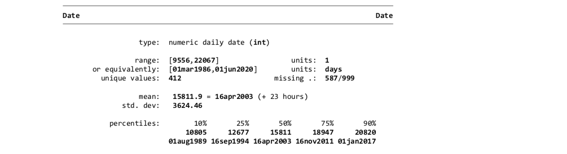
# display details of variable 'Date'
codebook DateIt can be observed that the ‘Date’ variable has units ‘days’ while actually it is recorded monthly.
# replace unit of 'Date' with month
replace Date = mofd(Date)
format %tm Date
tsset Date, monthly
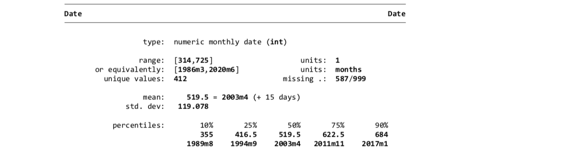
codebook DateThe ‘Date’ variable now has units ‘months’ which is correct.
3.2.1 Transformation from levels to first differences
The APT posits that the stock returns can be explained by reference to the unexpected changes in the macroeconomic variables rather than their levels.
Why should we shift to first differences rather than levels? This is required as we are dealing with a dynamic model here. Dynamic model is a model where the current value of yt depends on previous values of y or on previous values of one or more of the variables, eg., yt=β1+β2 x1t+β3x2t+β4x3t+β5x4t+⋯+γ1 y(t-1)+γ2x(1t-1)+⋯+γk x(kt-1)+ut
The current value of the stock return depends on previous values of stock along with other variables. This makes the errors to be correlated with one another, violating one of the assumption of Classical Linear Regression Model (CLRM). The errors are said to be ‘autocorrelated’ in this case. A potential remedy for autocorrelated residuals would be to switch to a model in first differences rather than in levels.
What are unexpected changes in the macroeconomic variables? The unexpected value of a variable can be defined as the difference between the actual (realised) value of the variable and its expected value. The question then arises that what is the expected value of the variables? It can be assumed that the investors have naive expectations that the next period value of the variable is equal to the current value. This being the case, the entire change in the variable from one period to the next is the unexpected change (because investors are assumed to expect no change). The first stage is to generate a set of changes or differences for each of the variables.
Target variable The variable whose behaviour we seek to explain is the ‘excess rate of return of the Microsoft stock’ in percentage. To find this, first we find the rate of return of Microsoft stock. For purposes of business analysis, small changes in the natural log of a variable are directly interpretable as rate of change, to a very close approximation. Hence, we calculate the difference in the natural log of the variable and multiply it with 100 to get the rate of return in percentage.
rmsoft = 100 * (ln (MICROSOFT / L.MICROSOFT) )
Next step is to find the ‘excess rate of reurn’ of Microsoft stock. The excess rate of return of the stock is given by subtracting the risk free rate from the rate of the stock. The US treasury bill yield of 3 months maturity (USTB3M) is usually taken as the risk free rate. The monthly risk free rate is given by:
mustb3m = USTB3M / 12
Excess rate of return of the Microsoft stock is given by:
ermsoft = rmsoft – mustb3m
The STATA codes are:
generate rmsoft = 100*(ln(MICROSOFT/L.MICROSOFT))
generate mustb3m=USTB3M/12
generate ermsoft=rmsoft-mustb3m
Predictors As mentioned earlier (refer Table 1), there are seven macroeconomic variables which act as preditors in this regression model.
- S&P 500: Excess return of S&P 500 stock contribute towards explaining the excess return of the target stock. As in the case of target variable, first we find the rate of retrun of S&P500.
rsandp=100 * (ln (MICROSOFT/L.MICROSOFT) ) Excess return of S&P 500 is given by:
*ersandp = rsandp - mustb3m *
- Inflation: Small changes in the natural log of a variable CPI is directly interpretable as inflation. inflation = 100 * (ln (CPI/L.CPI) ). The first difference is given by:
dinflation = inflation-L.inflation
- Industrial Production: The first difference of the variable is given by:
dprod = INDPRO - L.INDPRO
- Term spread: is given by term = USTB10Y - USTB3M. The first difference is given by:
rterm=term-L.term
- Consumer credit: is given by:
dcredit = CCREDIT - L.CCREDIT
- Credit spread: is given by:
dspread = BMINUSA - L.BMINUSA
- Money supply is given by:
dmoney = M1SUPPLY - L.M1SUPPLY
STATA code:
generate rsandp = 100*(ln(SANDP/L.SANDP))
generate ersandp=rsandp-mustb3m

generate inflation = 100*(ln(CPI/L.CPI))
generate dinflation = inflation-L.inflation

generate dprod = INDPRO-L.INDPRO

generate term = USTB10Y-L.USTB3M
generate rterm=term-L.term

generate dcredit = CCREDIT-L.CCREDIT
generate dspread = BMINUSA-L.BMINUSA
generate dmoney = M1SUPPLY-L.M1SUPPLY
3.3 Regression Analysis
We can now ready run the regression.
regress ermsoft ersandp rterm dpro dcredit dinflation dmoney dspreadThe output of regression is given below:
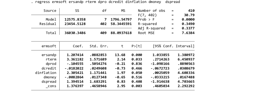
Note that the signs of the coefficients estimates match with the expected impact of the variable given in table 1. It can be observed that variables ersandp, rterm and dinflation have significant impact on ermsoft while variables dprod, dcredit, dmoney and dspread do not have significant influence on the target variable.
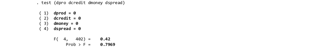
An F-test to verify the null hypothesis that variables dprod, dcredit, dmoney and dspread do not have significant impact on ermsoft is performed.
test (dpro dcredit dmoney dspread)The result suggests that the null hypothesis cannot be rejected. Hence, we can confirm that dprod, dcredit, dmoney and dspread do not have significant impact on ermsoft
4. The model
The model can be reduced as:
ermsoft_t = 1.33 + 1.28 ersand_t + 2.19 dinflation_t + 4.73 rterm_t + u_t
Using this model the fair market price of Microsoft stock can be estimated. In the event the market misprices the stock, the arbitrage opportunity can be harnessed to gain.
References
- https://www.investopedia.com
- https://en.wikipedia.org
- Book- ‘Introductory Econometrics for Finance’ (fourth edition) by Chris Brooks
- Book- ‘STATA guide to accompany Introductory Econometrics for Finance’ (fourth edition) by Lisa Schopohl, Robert Wichmann, Chris Brooks
- Blog post on ‘How to Model Gold Price’ by Alex Kim