Credit Risk Assessment
Loans form an integral part of banking operations. However, not all the loans are promptly returned and hence it is important for a bank to closely monitor its loan applications. This project is an analysis of the German credit dataset from the UCI Machine Learning repository. The dataset contains details of 1000 loan applicants with 21 attributes along with the classification as good or bad credit.
In this project, the relationship between the credit risk and various attributes will be explored through basic statistical techniques and presented through visualizations.
Contents
- Import data
- Data preparation, cleaning
- Exploratory data analysis
- Feature engineering
- Models
- Model evaluation
- Conclusion
- References
1. Import data
Let’s begin by downloading the data from the UCI Machine Learning repository.
from urllib.request import urlretrieve
urlretrieve('http://archive.ics.uci.edu/ml/machine-learning-databases/statlog/german/german.data', 'german.data')
('german.data', <http.client.HTTPMessage at 0x7effdfbb5550>)
The dataset has been downloaded and extracted.
2. Data Preparation and Cleaning
In this step, we do data preparation and cleaning, making the data suitable for subsequent analysis.
2.1 Load data into dataframe
The datafile is in .data format, delimited with space, and has no headers.
import pandas as pd
german_df = pd.read_csv('http://archive.ics.uci.edu/ml/machine-learning-databases/statlog/german/german.data',
                        delimiter=' ',header=None)
Now, let’s have an overview of the dataset.
german_df.info()
<class 'pandas.core.frame.DataFrame'>
RangeIndex: 1000 entries, 0 to 999
Data columns (total 21 columns):
 #   Column  Non-Null Count  Dtype
---  ------  --------------  -----
 0   0       1000 non-null   object
 1   1       1000 non-null   int64
 2   2       1000 non-null   object
 3   3       1000 non-null   object
 4   4       1000 non-null   int64
 5   5       1000 non-null   object
 6   6       1000 non-null   object
 7   7       1000 non-null   int64
 8   8       1000 non-null   object
 9   9       1000 non-null   object
 10  10      1000 non-null   int64
 11  11      1000 non-null   object
 12  12      1000 non-null   int64
 13  13      1000 non-null   object
 14  14      1000 non-null   object
 15  15      1000 non-null   int64
 16  16      1000 non-null   object
 17  17      1000 non-null   int64
 18  18      1000 non-null   object
 19  19      1000 non-null   object
 20  20      1000 non-null   int64
dtypes: int64(8), object(13)
memory usage: 164.2+ KB
The dataset contains 21 variables and 1000 observations. 8 variables are of numeric type and 13 of object type. As the object type variables do not have any null values, we can conclude that they are of categorical type.
2.2 Label the columns
Next, let’s label the variables for ease of use. The document describing the dataset may be referred for this.
urlretrieve('http://archive.ics.uci.edu/ml/machine-learning-databases/statlog/german/german.doc', 'german.doc')
f = open('german.doc')
german_doc= f.read()
print(german_doc)
Description of the German credit dataset.

1. Title: German Credit data

2. Source Information

Professor Dr. Hans Hofmann
Institut f"ur Statistik und "Okonometrie
Universit"at Hamburg
FB Wirtschaftswissenschaften
Von-Melle-Park 5
2000 Hamburg 13

3. Number of Instances:  1000

Two datasets are provided.  the original dataset, in the form provided
by Prof. Hofmann, contains categorical/symbolic attributes and
is in the file "german.data".

For algorithms that need numerical attributes, Strathclyde University
produced the file "german.data-numeric".  This file has been edited
and several indicator variables added to make it suitable for
algorithms which cannot cope with categorical variables.   Several
attributes that are ordered categorical (such as attribute 17) have
been coded as an integer.    This was the form used by StatLog.


6. Number of Attributes german: 20 (7 numerical, 13 categorical)
   Number of Attributes german.numer: 24 (24 numerical)


7.  Attribute description for german

Attribute 1:  (qualitative)
	       Status of existing checking account
               A11 :      ... <    0 DM
	       A12 : 0 <= ... <  200 DM
	       A13 :      ... >= 200 DM /
		     salary assignments for at least 1 year
               A14 : no checking account

Attribute 2:  (numerical)
	      Duration in month

Attribute 3:  (qualitative)
	      Credit history
	      A30 : no credits taken/
		    all credits paid back duly
              A31 : all credits at this bank paid back duly
	      A32 : existing credits paid back duly till now
              A33 : delay in paying off in the past
	      A34 : critical account/
		    other credits existing (not at this bank)

Attribute 4:  (qualitative)
	      Purpose
	      A40 : car (new)
	      A41 : car (used)
	      A42 : furniture/equipment
	      A43 : radio/television
	      A44 : domestic appliances
	      A45 : repairs
	      A46 : education
	      A47 : (vacation - does not exist?)
	      A48 : retraining
	      A49 : business
	      A410 : others

Attribute 5:  (numerical)
	      Credit amount

Attribute 6:  (qualitative)
	      Savings account/bonds
	      A61 :          ... <  100 DM
	      A62 :   100 <= ... <  500 DM
	      A63 :   500 <= ... < 1000 DM
	      A64 :          .. >= 1000 DM
              A65 :   unknown/ no savings account

Attribute 7:  (qualitative)
	      Present employment since
	      A71 : unemployed
	      A72 :       ... < 1 year
	      A73 : 1  <= ... < 4 years
	      A74 : 4  <= ... < 7 years
	      A75 :       .. >= 7 years

Attribute 8:  (numerical)
	      Installment rate in percentage of disposable income

Attribute 9:  (qualitative)
	      Personal status and sex
	      A91 : male   : divorced/separated
	      A92 : female : divorced/separated/married
              A93 : male   : single
	      A94 : male   : married/widowed
	      A95 : female : single

Attribute 10: (qualitative)
	      Other debtors / guarantors
	      A101 : none
	      A102 : co-applicant
	      A103 : guarantor

Attribute 11: (numerical)
	      Present residence since

Attribute 12: (qualitative)
	      Property
	      A121 : real estate
	      A122 : if not A121 : building society savings agreement/
				   life insurance
              A123 : if not A121/A122 : car or other, not in attribute 6
	      A124 : unknown / no property

Attribute 13: (numerical)
	      Age in years

Attribute 14: (qualitative)
	      Other installment plans
	      A141 : bank
	      A142 : stores
	      A143 : none

Attribute 15: (qualitative)
	      Housing
	      A151 : rent
	      A152 : own
	      A153 : for free

Attribute 16: (numerical)
              Number of existing credits at this bank

Attribute 17: (qualitative)
	      Job
	      A171 : unemployed/ unskilled  - non-resident
	      A172 : unskilled - resident
	      A173 : skilled employee / official
	      A174 : management/ self-employed/
		     highly qualified employee/ officer

Attribute 18: (numerical)
	      Number of people being liable to provide maintenance for

Attribute 19: (qualitative)
	      Telephone
	      A191 : none
	      A192 : yes, registered under the customers name

Attribute 20: (qualitative)
	      foreign worker
	      A201 : yes
	      A202 : no


8.  Cost Matrix

This dataset requires use of a cost matrix (see below)


      1        2
----------------------------
  1   0        1
-----------------------
  2   5        0

(1 = Good,  2 = Bad)

the rows represent the actual classification and the columns
the predicted classification.

It is worse to class a customer as good when they are bad (5),
than it is to class a customer as bad when they are good (1).
Based on the description, we name the columns.
german_df.columns=['account_bal','duration','payment_status','purpose',
                   'credit_amount','savings_bond_value','employed_since',
                   'intallment_rate','sex_marital','guarantor','residence_since',
                   'most_valuable_asset','age','concurrent_credits','type_of_housing',
                   'number_of_existcr','job','number_of_dependents','telephon',
                   'foreign','target']
german_df= german_df.replace(['A11','A12','A13','A14', 'A171','A172','A173','A174','A121','A122','A123','A124'],['neg_bal','positive_bal','positive_bal','no_acc','unskilled','unskilled','skilled','highly_skilled',
'none','car','life_insurance','real_estate'])
3. Exploratory Data Analysis and Visualization
# import libraries for visualizations

import numpy as np
import seaborn as sns
import matplotlib
import matplotlib.pyplot as plt
%matplotlib inline

sns.set_style('darkgrid')
matplotlib.rcParams['font.size'] = 14
matplotlib.rcParams['figure.figsize'] = (9, 5)
matplotlib.rcParams['figure.facecolor'] = '#00000000'
3.1 Examine missing values
# check for missing values
german_df.isna().any().any()
False
3.1 Examine distribution of target column
german_df.target.unique()
array([1, 2])
The target column has two values:
- 1: representing a good loan
- 2: representing a bad (defaulted) loan.
The usual convention is to use ‘1’ for bad loans and ‘0’ for good loans. Let’s replace the values to comply to the convention.
from sklearn.preprocessing import LabelEncoder

le= LabelEncoder()
le.fit(german_df.target)
german_df.target=le.transform(german_df.target)
german_df.target.head(5)
0    0
1    1
2    0
3    0
4    1
Name: target, dtype: int64
An understanding of the percentage of good and bad loans would be useful for further analysis. A pie chart would be the best tool to help with this.
good_bad_per=round(((german_df.target.value_counts()/german_df.target.count())*100))
good_bad_per
plt.pie(good_bad_per,labels=['Good loans', 'Bad loans'], autopct='%1.0f%%', startangle=90)
plt.title('Percentage of good and bad loans');
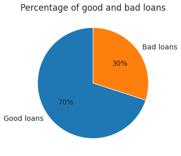
The pie chart shows that 30% of the loan applicants defaulted. From this information, we see that this is an imbalanced class problem. Hence, we will have to weigh the classes by their representation in the data to reflect this imbalance.
4.2 Exploration of continues variables
- Summary statistics
- Histograms
- Box-plots
Observations
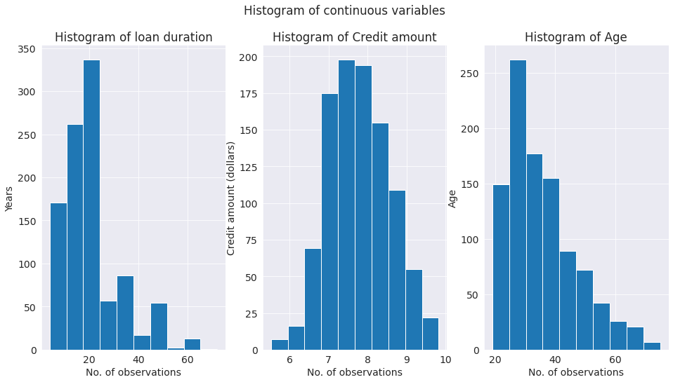
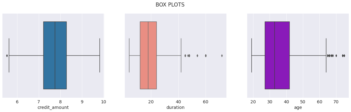
- A glance of the distribution of the continues variables shows that there is a wide gap in the range of variables. The credit amount variable might have to be transformed to bring all variables to similar range.
- The histogram suggests that the credit amount is approximately normally distributed. However, age and duration have a skewed distribution.
- The box plots show that most of the credits amounts are between 1000 to 4500 dollars. The credit amount is positively skewed. Most of the loan duration is from 15 to 30 months. Majority of the loan applicants have age between 28 - 43.
german_df[['credit_amount','duration','age']].describe()
| credit_amount | duration | age | |
|---|---|---|---|
| count | 1000.000000 | 1000.000000 | 1000.000000 |
| mean | 3271.258000 | 20.903000 | 35.546000 |
| std | 2822.736876 | 12.058814 | 11.375469 |
| min | 250.000000 | 4.000000 | 19.000000 |
| 25% | 1365.500000 | 12.000000 | 27.000000 |
| 50% | 2319.500000 | 18.000000 | 33.000000 |
| 75% | 3972.250000 | 24.000000 | 42.000000 |
| max | 18424.000000 | 72.000000 | 75.000000 |
german_df['credit_amount']=np.log(german_df['credit_amount'])
german_df[['credit_amount','duration','age']].describe()
| credit_amount | duration | age | |
|---|---|---|---|
| count | 1000.000000 | 1000.000000 | 1000.000000 |
| mean | 7.788691 | 20.903000 | 35.546000 |
| std | 0.776474 | 12.058814 | 11.375469 |
| min | 5.521461 | 4.000000 | 19.000000 |
| 25% | 7.219276 | 12.000000 | 27.000000 |
| 50% | 7.749107 | 18.000000 | 33.000000 |
| 75% | 8.287088 | 24.000000 | 42.000000 |
| max | 9.821409 | 72.000000 | 75.000000 |
# histograms of continues variables

fig, axes = plt.subplots(1,3, figsize=(16,8))
plt.suptitle('Histogram of continuous variables')
axes[0].hist(german_df['duration'])
axes[0].set_xlabel('No. of observations')
axes[0].set_ylabel('Years')
axes[0].set_title('Histogram of loan duration');

axes[1].hist(german_df['credit_amount'])
axes[1].set_xlabel('No. of observations')
axes[1].set_ylabel('Credit amount (dollars)')
axes[1].set_title('Histogram of Credit amount');

axes[2].hist(german_df['age'])
axes[2].set_xlabel('No. of observations')
axes[2].set_ylabel('Age')
axes[2].set_title('Histogram of Age');
# box-plots of continues variables

fig, ax = plt.subplots(1,3,figsize=(20,5))
plt.suptitle('BOX PLOTS')
sns.boxplot(german_df['credit_amount'], ax=ax[0]);
sns.boxplot(german_df['duration'], ax=ax[1], color='salmon');
sns.boxplot(german_df['age'], ax=ax[2], color='darkviolet');
/usr/local/lib/python3.7/dist-packages/seaborn/_decorators.py:43: FutureWarning: Pass the following variable as a keyword arg: x. From version 0.12, the only valid positional argument will be `data`, and passing other arguments without an explicit keyword will result in an error or misinterpretation.
  FutureWarning
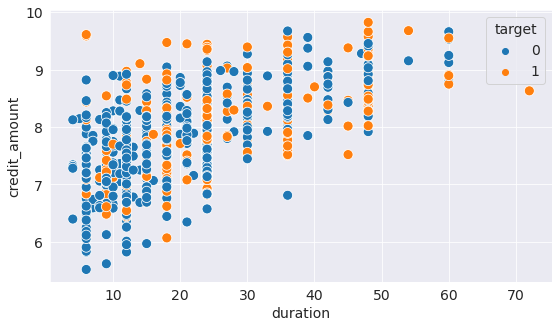
4.2 Relationship between the credit amount and repayment duration
- scatter plot
Observations
The scatter plot shows that in general, larger loans have longer duration of repayment. Cases where large loans are given with short repayment period have turned out to be bad loans.
sns.scatterplot(y=german_df.credit_amount,
                x=german_df.duration,
                hue=german_df.target,
                s=100,
                );
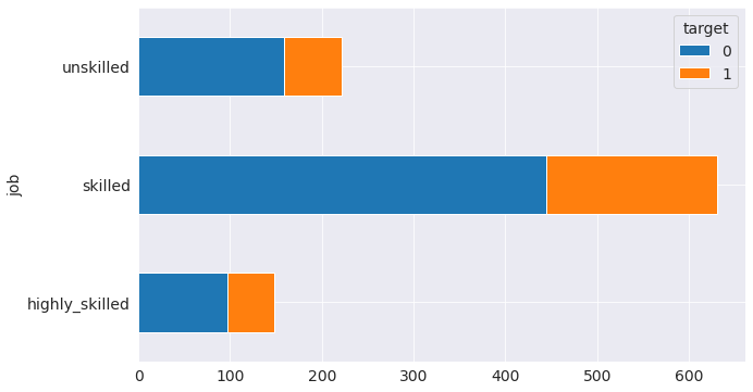
4.3 Exploration of categorical variables
Relationship between credit risk and skills of loan applicant
- Bar-graph
Observations
The graph shows that candidates who are unemployed/unskilled pose a high risk
german_df.groupby('job')['target'].value_counts().unstack(level=1).plot.barh(stacked=True, figsize=(10, 6))
<matplotlib.axes._subplots.AxesSubplot at 0x7effccf2f210>
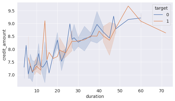
4.4 Relationship between credit amount and duration of the loan
- Line graph
Observation
There is a linear relationship between the credit amount and duration. The larger the credit amount, the longer the repayment duration is.
sns.lineplot(data=german_df, x='duration', y='credit_amount', hue='target', palette='deep');
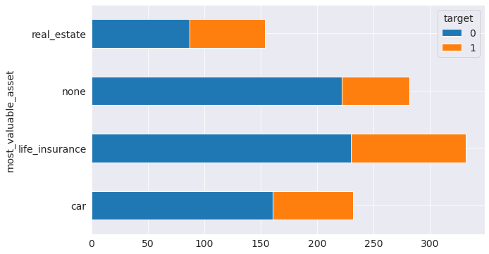
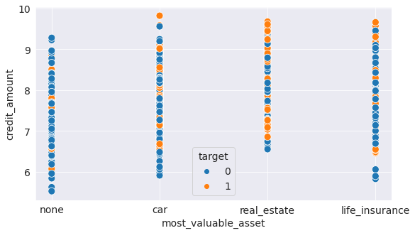
4.5 Relationship between the most valuable asset of the candidate and the credit amount, credit risk
- stacked bar chart
- scatter plot
The categorical coding used in the graphs is:
- A121 : real estate
- A122 : if not A121 : building society savings agreement/life insurance
- A123 : if not A121/A122 : car or other, not in attribute 6
- A124 : unknown / no property
Observations
The graphs show that people with real estate assets are very risky.
german_df.groupby('most_valuable_asset')['target'].value_counts().unstack(level=1).plot.barh(stacked=True, figsize=(10, 6))
<matplotlib.axes._subplots.AxesSubplot at 0x7effcce61d90>
sns.scatterplot(y=german_df.credit_amount,
                x=german_df.most_valuable_asset,
                hue=german_df.target,
                s=100,
                );
4. Encode categorical variables
Most machine learning models cannot deal with categorical variables. So, we need to encode the 13 categorical variables that we have in the German dataset.
# Number of unique classes in each object column
german_df.select_dtypes('object').apply(pd.Series.nunique, axis = 0)
account_bal             3
payment_status          5
purpose                10
savings_bond_value      5
employed_since          5
sex_marital             4
guarantor               3
most_valuable_asset     4
concurrent_credits      3
type_of_housing         3
job                     3
telephon                2
foreign                 2
dtype: int64
We have categorical variables of 2 to 10 categories. We go for Label encoding for variables with only two categories where as for variables with more than two categories, we go for one-hot encoding. In label encoding, we assign each unique category in a categorical variable with an integer. No new columns are created. In one-hot encoding, we create a new column for each unique category in a categorical variable. The only downside to one-hot encoding is that the number of features (dimensions of the data) can explode with categorical variables with many categories. To deal with this, we can perform one-hot encoding followed by PCA or other dimensionality reduction methods to reduce the number of dimensions (while still trying to preserve information).
For label encoding, we use the Scikit-Learn LabelEncoder and for one-hot encoding, the pandas get_dummies(df) function.
# sklearn preprocessing for dealing with categorical variables
from sklearn.preprocessing import LabelEncoder

# Create a label encoder object
le = LabelEncoder()
le_count = 0

# Iterate through the columns
for col in german_df:
    if german_df[col].dtype == 'object':
        # If 2 or fewer unique categories
        if len(list(german_df[col].unique())) <= 2:
            # Train on the training data
            le.fit(german_df[col])
            # Transform both training and testing data
            german_df[col] = le.transform(german_df[col])

            # Keep track of how many columns were label encoded
            le_count += 1

print('%d columns were label encoded.' % le_count)
2 columns were label encoded.
# one-hot encoding of categorical variables
german_df = pd.get_dummies(german_df)

print('Encoded Features shape: ', german_df.shape)
Encoded Features shape: (1000, 58)
Now that we have encoded the variables, let’s continue with the EDA.
4.1 Correlation between the variables
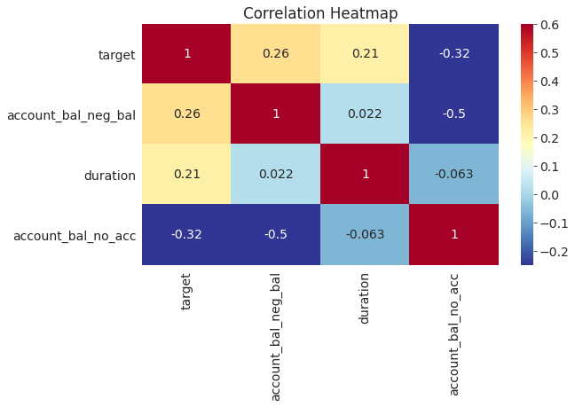
Let’s look at correlations between the features and the target using Pearson correlation coefficient. In this case, a positive correlation represents correlation with credit default while a negative correlation represents correlation with credit repayment.
Observations:
Positive correlation:
-
People with checking accounts with a negative balance (
account_bal_A11) are likely to default the loan. -
Longer duration loans (
duration) tend to be defaulted.
Negative correlation:
- People with no checking account (
account_bal_A14) are likely to repay the loan.
# Find correlations with the target and sort
correlations = german_df.corr()['target'].sort_values()

# Display correlations
print('Most Positive Correlations:\n', correlations.tail(15))
print('\nMost Negative Correlations:\n', correlations.head(15))
Most Positive Correlations:
 sex_marital_A92                    0.075493
type_of_housing_A153               0.081556
account_bal_positive_bal           0.089895
type_of_housing_A151               0.092785
concurrent_credits_A141            0.096510
purpose_A40                        0.096900
employed_since_A72                 0.106397
credit_amount                      0.109570
most_valuable_asset_real_estate    0.125750
payment_status_A31                 0.134448
payment_status_A30                 0.144767
savings_bond_value_A61             0.161007
duration                           0.214927
account_bal_neg_bal                0.258333
target                             1.000000
Name: target, dtype: float64

Most Negative Correlations:
 account_bal_no_acc         -0.322436
payment_status_A34         -0.181713
type_of_housing_A152       -0.134589
savings_bond_value_A65     -0.129238
most_valuable_asset_none   -0.119300
concurrent_credits_A143    -0.113285
purpose_A43                -0.106922
purpose_A41                -0.099791
age                        -0.091127
savings_bond_value_A64     -0.085749
foreign                    -0.082079
sex_marital_A93            -0.080677
employed_since_A74         -0.075980
savings_bond_value_A63     -0.070954
employed_since_A75         -0.059733
Name: target, dtype: float64
Let’s look at the heatmap of significant correlations.
# Extract the significantly correlated variables
corr_data = german_df[['target', 'account_bal_neg_bal','duration','account_bal_no_acc']]
corr_data_corrs = corr_data.corr()


# Heatmap of correlations
sns.heatmap(corr_data_corrs, cmap = plt.cm.RdYlBu_r, vmin = -0.25, annot = True, vmax = 0.6)
plt.title('Correlation Heatmap');
5. Feature engineering
Feature engineering refers to creating most useful features out of the data. This represents one of the patterns in machine learning: feature engineering has a greater return on investment than model building and hyperparameter tuning. [Source]
Feature engineering refers to a general process and can involve both feature construction: adding new features from the existing data, and feature selection: choosing only the most important features or other methods of dimensionality reduction. There are many techniques we can use to both create features and select features.
For this problem, we will try to construct polynomial features.
Polynomial Features
Here, we find interactions between significant features. The correlation between the interaction features and the target is checked. If the interaction features are found to have greater correlation with the target compared to the original features, they are included in the machine learning model as they can help the model learn better.
# Make a new dataframe for polynomial features
poly_features = german_df[['duration','account_bal_neg_bal','account_bal_no_acc']]
poly_target=german_df['target']

from sklearn.preprocessing import PolynomialFeatures

# Create the polynomial object with specified degree
poly_transformer = PolynomialFeatures(degree = 2)
# Train the polynomial features
poly_transformer.fit(poly_features)

# Transform the features
poly_features = poly_transformer.transform(poly_features)
print('Polynomial Features shape: ', poly_features.shape)
Polynomial Features shape: (1000, 10)
This creates a considerable number of new features. To get the names we have to use the polynomial features get_feature_names method.
poly_transformer.get_feature_names(input_features = ['duration','account_bal_neg_bal','account_bal_no_acc'])
['1',
 'duration',
 'account_bal_neg_bal',
 'account_bal_no_acc',
 'duration^2',
 'duration account_bal_neg_bal',
 'duration account_bal_no_acc',
 'account_bal_neg_bal^2',
 'account_bal_neg_bal account_bal_no_acc',
 'account_bal_no_acc^2']
Now, we can see whether any of these new features are correlated with the target.
# Create a dataframe for polynomial features
poly_features = pd.DataFrame(
    poly_features, columns = poly_transformer.get_feature_names(
        ['duration','account_bal_neg_bal','account_bal_no_acc']))

# Add in the target
poly_features['target'] = poly_target

# Find the correlations with the target
poly_corrs = poly_features.corr()['target'].sort_values()

# Display the correlations
poly_corrs
account_bal_no_acc                       -0.322436
account_bal_no_acc^2                     -0.322436
duration account_bal_no_acc              -0.232697
duration^2                                0.200996
duration                                  0.214927
account_bal_neg_bal                       0.258333
account_bal_neg_bal^2                     0.258333
duration account_bal_neg_bal              0.303343
target                                    1.000000
1                                              NaN
account_bal_neg_bal account_bal_no_acc         NaN
Name: target, dtype: float64
All the new variables have a greater (in terms of absolute magnitude) correlation with the target than the original features. We will add these features to a copy of the German dataset and then evaluate models with and without the features.
list(poly_features)
['1',
 'duration',
 'account_bal_neg_bal',
 'account_bal_no_acc',
 'duration^2',
 'duration account_bal_neg_bal',
 'duration account_bal_no_acc',
 'account_bal_neg_bal^2',
 'account_bal_neg_bal account_bal_no_acc',
 'account_bal_no_acc^2',
 'target']
# deleting duplicate columns in poly_features

for i in list(poly_features.columns):
  for j in list(german_df.columns):
    if (i==j):
      poly_features.drop(labels=i, axis=1, inplace=True)

poly_features.drop(labels='1', axis=1, inplace=True)
list(poly_features)
['duration^2',
 'duration account_bal_neg_bal',
 'duration account_bal_no_acc',
 'account_bal_neg_bal^2',
 'account_bal_neg_bal account_bal_no_acc',
 'account_bal_no_acc^2']
# Print shape of original german_df
print('Original features shape: ', german_df.shape)

# Merge polynomial features into the dataframe
german_df_poly = german_df.merge(poly_features, left_index=True, right_index=True, how = 'left')

# Print out the new shapes
print('Merged polynomial features shape: ', german_df_poly.shape)
Original features shape:  (1000, 58)
Merged polynomial features shape:  (1000, 64)
german_df_poly.isna().any().any()
False
list(german_df_poly)
['duration',
 'credit_amount',
 'intallment_rate',
 'residence_since',
 'age',
 'number_of_existcr',
 'number_of_dependents',
 'telephon',
 'foreign',
 'target',
 'account_bal_neg_bal',
 'account_bal_no_acc',
 'account_bal_positive_bal',
 'payment_status_A30',
 'payment_status_A31',
 'payment_status_A32',
 'payment_status_A33',
 'payment_status_A34',
 'purpose_A40',
 'purpose_A41',
 'purpose_A410',
 'purpose_A42',
 'purpose_A43',
 'purpose_A44',
 'purpose_A45',
 'purpose_A46',
 'purpose_A48',
 'purpose_A49',
 'savings_bond_value_A61',
 'savings_bond_value_A62',
 'savings_bond_value_A63',
 'savings_bond_value_A64',
 'savings_bond_value_A65',
 'employed_since_A71',
 'employed_since_A72',
 'employed_since_A73',
 'employed_since_A74',
 'employed_since_A75',
 'sex_marital_A91',
 'sex_marital_A92',
 'sex_marital_A93',
 'sex_marital_A94',
 'guarantor_A101',
 'guarantor_A102',
 'guarantor_A103',
 'most_valuable_asset_car',
 'most_valuable_asset_life_insurance',
 'most_valuable_asset_none',
 'most_valuable_asset_real_estate',
 'concurrent_credits_A141',
 'concurrent_credits_A142',
 'concurrent_credits_A143',
 'type_of_housing_A151',
 'type_of_housing_A152',
 'type_of_housing_A153',
 'job_highly_skilled',
 'job_skilled',
 'job_unskilled',
 'duration^2',
 'duration account_bal_neg_bal',
 'duration account_bal_no_acc',
 'account_bal_neg_bal^2',
 'account_bal_neg_bal account_bal_no_acc',
 'account_bal_no_acc^2']
6. Data split to train and test datasets
As the German dataset is an imbalanced dataset with more number repayors compared to defaulters, we used stratified random test_train_split to split the dataset into random test and train datasets so that relative class frequencies are preserved.
from sklearn.model_selection import train_test_split
x, y = german_df.drop('target', axis=1), german_df['target']
x.shape, y.shape
((1000, 57), (1000,))
x_train, x_test, y_train, y_test= train_test_split(x,y, test_size=.2, random_state=42, stratify=y)
x_train.shape, x_test.shape
((800, 57), (200, 57))
x_train
y_train
828    1
997    0
148    0
735    0
130    0
      ..
492    0
545    1
298    0
417    0
749    0
Name: target, Length: 800, dtype: int64
# train and test split on german_df_poly
X, Y = german_df_poly.drop('target', axis=1), german_df_poly['target']
print(X.shape, Y.shape)

X_train, X_test, Y_train, Y_test= train_test_split(X,Y, test_size=.2, random_state=42, stratify=Y)
(1000, 63) (1000,)
7. Models
Evaluation criteria
Let’s have a look at the different options available.
| Evaluation criteria | Description |
|---|---|
| Accuracy | (true positive+ true negative) / total obs |
| Precision | true positive/ total predicted positive |
| Recall | true positive/ total actual positive |
| F1 | 2* precision * recall / (precision + recall) |
| AUC ROC | Area Under ROC Curve (TPR Vs. FPR for all classification thresholds) |
-
Accuracy: The German dataset is an imbalanced dataset. Accuracy would give a high score by predicting the majority class but would fail to predict the minority class, which is the defaulters. Hence, this is not a suitable metric for this dataset.
-
Precision: Precision is a good metric when the costs of false positive are high. Example, email spam detection.
-
Recall: This metric is suitable when the costs of false negative are high. Example, predicting a defaulter as not defaulter. This costs a huge loss for the bank. Hence, this is a suitable metric for our case.
-
F1: measure of both precision and recall.
- AUC ROC: It is the plot of TPR vs FPR. All other criteria discussed here assume 0.5 as the decision threshold for the classification. However, it may not be always true. The AUC helps us evaluate the performance of the model for all classification thresholds. The higher the value of the AUC metric, the better the model.
- True positive rate (TPR) = TP/ Total actual positive
- False positive rate (FPR) = FP/ Total actual negative
We will use Recall and AUC ROC as evaluation metric.
Baseline
y.value_counts(normalize=True)
0    0.7
1    0.3
Name: target, dtype: float64
It means that the baseline accuracy is 70%, i.e., even if we classify all the samples as defaulters, we will be 70% accurate.
Models without tuning
# import packages, functions, and classes
from sklearn.ensemble import RandomForestClassifier
from sklearn.linear_model import LogisticRegression
from sklearn.tree import DecisionTreeClassifier
from sklearn.neighbors import KNeighborsClassifier
from xgboost import XGBClassifier

from sklearn.metrics import roc_auc_score, recall_score, classification_report
from sklearn.model_selection import StratifiedKFold, cross_val_score, cross_validate
# prepare models
models = []
models.append(('DT', DecisionTreeClassifier(random_state=42)))
models.append(('LR', LogisticRegression(random_state=42)))
models.append(('RF', RandomForestClassifier(random_state=42)))
models.append(('XGB', XGBClassifier(random_state=42)))
models.append(('KNN', KNeighborsClassifier()))

# evaluate each model in turn
results_recall = []
results_roc_auc= []
names = []
# recall= tp/ (tp+fn). Best value=1, worst value=0
scoring = ['recall', 'roc_auc']

for name, model in models:
        # split dataset into k folds. use one-fold for validation and remaining k-1 folds for training
        skf= StratifiedKFold(n_splits=10, shuffle=True, random_state=42)
        # Evaluate a score by cross-validation. Returns array of scores of the model for each run of the cross validation.
        #cv_results = cross_val_score(model, x_train, y_train, cv=skf, scoring=scoring)
        cv_results = cross_validate(model, x_train, y_train, cv=skf, scoring=scoring)
        results_recall.append(cv_results['test_recall'])
        results_roc_auc.append(cv_results['test_roc_auc'])
        names.append(name)
        msg = "%s- recall:%f roc_auc:%f" % (name, cv_results['test_recall'].mean(),cv_results['test_roc_auc'].mean())
        print(msg)

# boxplot algorithm comparison
#recall score plots
fig = plt.figure(figsize=(11,6))
fig.suptitle('Recall scoring Comparison')
ax = fig.add_subplot(111)
plt.boxplot(results_recall, showmeans=True)
ax.set_xticklabels(names)
plt.show();
# roc auc score box plots
fig = plt.figure(figsize=(11,6))
fig.suptitle('AUC scoring Comparison')
ax = fig.add_subplot(111)
plt.boxplot(results_roc_auc, showmeans=True)
ax.set_xticklabels(names)
plt.show();
Gaussian NB model has the highest roc_auc score. However, Logistic regression, Randon forests and XGBoost has a better AUC score than Gaussian NB. Now let us tune hyperparameters for each of these models.
from sklearn.metrics import accuracy_score, confusion_matrix, roc_auc_score, recall_score
from sklearn.model_selection import StratifiedKFold, cross_val_score
from sklearn.model_selection import GridSearchCV
7.2 Logistic regression
- first, fit on the original dataset set. Then, fit on polynomial features obtained by feature engineering
-
polynomial features gives better results. Hence, this dataset will be used for further exploration
- C: variable that controls regularization. Smaller values indicate higher regularization. It’s a penalty term that disincentivize overfitting
First let us choose between german_df and german_df_poly. Use C=0.0001 which is randomly chosen.
# Logistic model on data=german_df
log_reg = LogisticRegression(C = 0.0001, random_state=42)
log_reg.fit(x_train, y_train)
print('Dataset: german_df\n Recall score on train set: {:.2f}'.format(cross_val_score(log_reg, x_train, y_train, cv=skf, scoring='recall').mean()))

# Logistic model on data=german_df_poly
log_reg_poly = LogisticRegression(C = 0.0001, random_state=42, solver='lbfgs', max_iter=1000)
log_reg_poly.fit(X_train, Y_train)
print('Dataset: german_df_poly\n Recall score on train set: {:.2f}'.format(cross_val_score(log_reg_poly, X_train, Y_train, cv=skf, scoring='recall').mean()))
Dataset: german_df
 Recall score on train set: 0.01
Dataset: german_df_poly
 Recall score on train set: 0.18
We see considerable improvement in recall score with german_df_poly dataset. Hence, we proceed with german_df_poly for tuning regularization parameter C.
C=[1,0.1,0.01,0.001,0.0001]

# Create lists to save the values of recall score on training and test sets
train_recall = []
test_recall = []

for c in C:
  log_reg_poly = LogisticRegression(C = c, random_state=42, solver='lbfgs', max_iter=5000).fit(X_train, Y_train)
  train_recall.append(cross_val_score(log_reg_poly, X_test, Y_test, cv=skf,scoring='recall').mean())
  test_recall.append(recall_score(Y_test, log_reg_poly.predict(X_test)))

# plot graph of recall score vs. C
plt.plot(C, train_recall, label='train')
plt.plot(C, test_recall, label='test')
plt.legend()
plt.xlabel('C')
plt.ylabel('Recall score')
plt.title('Logistic regression: recall score vs C');
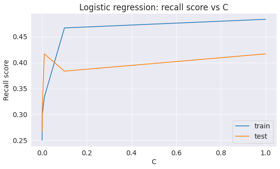
test_recall
[0.4166666666666667,
 0.38333333333333336,
 0.4166666666666667,
 0.31666666666666665,
 0.26666666666666666]
We get the maximum recall score on test set with overfitting at C=0.01
# Final logistic model
log_reg_poly = LogisticRegression(C = 0.01, random_state=42, solver='lbfgs', max_iter=5000).fit(X_train, Y_train)
print('Recall score on test dataset: {:.2f}'.format(recall_score(Y_test, log_reg_poly.predict(X_test))))
print('\nAUC ROC score on test dataset: {:.2f}'.format(roc_auc_score(Y_test,log_reg_poly.predict_proba(X_test)[:, 1])))
Recall score on test dataset: 0.42

AUC ROC score on test dataset: 0.78
7.3 Random Forest
- find optimal number of trees
- max depth
- min number of samples per leaf
- max features
Now, let’s try to improve this result. Let’s start with the number of trees.
# Create lists to save the values of accuracy on training and test sets
train_acc = []
test_acc = []
trees_grid = [5, 10, 15, 20, 30, 50, 75, 100]

for ntrees in trees_grid:
    rf = RandomForestClassifier(n_estimators=ntrees, random_state=42, n_jobs=-1).fit(X_train, Y_train)
    train_acc.append(cross_val_score(rf, X_train, Y_train, cv=skf, scoring='recall').mean())
    test_acc.append(recall_score(rf.predict(X_test), Y_test))
print("Best recall score on test dataset is {:.2f}% with {} trees".format(max(test_acc)*100,
                                                         trees_grid[np.argmax(test_acc)]))
# plot
plt.plot(trees_grid, train_acc, label='train')
plt.plot(trees_grid, test_acc, label='test')
plt.legend()
plt.xlabel('No. of trees (n_estimators)')
plt.ylabel('Accuracies (Recall score)')
plt.title('Random-Forest: accuracy vs n_estimators');
Best recall score on test dataset is 68.29% with 20 trees
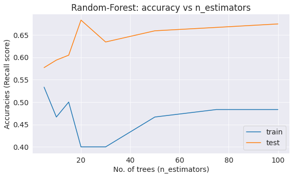
Best accuracy is achieved with 20 tress.
# Initialize the set of parameters for exhaustive search and fit
parameters = {'max_features': [7, 10, 16, 18],
              'min_samples_leaf': [1, 3, 5, 7],
              'max_depth': [15, 20, 24, 27]}
rf = RandomForestClassifier(n_estimators=20, random_state=42, n_jobs=-1)
gcv = GridSearchCV(rf, parameters, n_jobs=-1, cv=skf, verbose=1, scoring='recall')
gcv_fit= gcv.fit(X_train, Y_train)
Fitting 10 folds for each of 64 candidates, totaling 640 fits


[Parallel(n_jobs=-1)]: Using backend LokyBackend with 2 concurrent workers.
[Parallel(n_jobs=-1)]: Done  46 tasks      | elapsed:    5.5s
[Parallel(n_jobs=-1)]: Done 196 tasks      | elapsed:   22.1s
[Parallel(n_jobs=-1)]: Done 446 tasks      | elapsed:   49.8s
[Parallel(n_jobs=-1)]: Done 640 out of 640 | elapsed:  1.2min finished
# evaluate on train and test datasets
cross_val= cross_val_score(gcv_fit.best_estimator_, X_train, Y_train, cv=skf,scoring='recall').mean()
recall_sc=recall_score(Y_test,gcv_fit.best_estimator_.predict(X_test))
roc_sc= roc_auc_score(Y_test,gcv_fit.best_estimator_.predict_proba(X_test)[:, 1])
# print scores
print("GCV best parameters: ",gcv.best_params_)
print("GCV best score: {:.2f}".format(gcv.best_score_))
print("Cross val score on train dataset: {:.2f}".format(cross_val))
print("Recall score on test dataset: {:.2f}".format(recall_sc))
print("ROC AUC score on test dataset: {:.2f}".format(roc_sc))
GCV best parameters:  {'max_depth': 20, 'max_features': 18, 'min_samples_leaf': 3}
GCV best score: 0.48
Cross val score on train dataset: 0.48
Recall score on test dataset: 0.40
ROC AUC score on test dataset: 0.74
7.4 XGBoost
# Create lists to save the values of accuracy on training and test sets
train_acc = []
test_acc = []
estimator_grid = [5, 10, 15, 20, 30, 50, 75, 100]

for nestimator in estimator_grid:
    xg = XGBClassifier(n_estimators=nestimator, random_state=42, n_jobs=-1).fit(X_train, Y_train)
    train_acc.append(cross_val_score(xg, X_test, Y_test, cv=skf, scoring='recall').mean())
    test_acc.append(recall_score(xg.predict(X_test), Y_test))
print("Best recall score on test dataset is {:.2f}% with {} estimators".format(max(test_acc)*100,
                                                         estimator_grid[np.argmax(test_acc)]))
# plot
plt.plot(estimator_grid, train_acc, label='train')
plt.plot(estimator_grid, test_acc, label='test')
plt.legend()
plt.xlabel('No. of trees (n_estimators)')
plt.ylabel('Accuracies (Recall score)')
plt.title('XG-Boost: accuracy vs n_estimators');
Best recall score on test dataset is 66.67% with 10 estimators
#model
model_xg = XGBClassifier(random_state=42)
model_xg.fit(X_train, Y_train)
#evaluate
print('Train accuracy:', cross_val_score(model_xg, X_train, Y_train, cv=skf, scoring='recall').mean())
print('Recall score on test dataset:', recall_score(Y_test, model_xg.predict(X_test)))
print('ROC AUC score on test dataset:', roc_auc_score(Y_test, model_xg.predict_proba(X_test)[:,1]))
Train accuracy: 0.45
Recall score on test dataset: 0.5
ROC AUC score on test dataset: 0.7957142857142858
# Initialize the set of parameters for exhaustive search and fit
parameters = {'max_features': [7, 10, 16, 18],
              'min_samples_leaf': [1, 3, 5, 7],
              'max_depth': [15, 20, 24, 27]}
model_xg = XGBClassifier(n_estimators=10, random_state=42, n_jobs=-1)
gcv = GridSearchCV(model_xg, parameters, n_jobs=-1, cv=skf, verbose=1, scoring='recall')
gcv_fit= gcv.fit(X_train, Y_train)
Fitting 10 folds for each of 64 candidates, totaling 640 fits


[Parallel(n_jobs=-1)]: Using backend LokyBackend with 2 concurrent workers.
[Parallel(n_jobs=-1)]: Done  88 tasks      | elapsed:    4.6s
[Parallel(n_jobs=-1)]: Done 388 tasks      | elapsed:   20.1s
[Parallel(n_jobs=-1)]: Done 640 out of 640 | elapsed:   33.0s finished
gcv.best_params_, gcv.best_score_
({'max_depth': 15, 'max_features': 7, 'min_samples_leaf': 1}, 0.4625)
# evaluate on train and test datasets
cross_val= cross_val_score(gcv_fit.best_estimator_, X_train, Y_train, cv=skf,scoring='recall').mean()
recall_sc=recall_score(Y_test,gcv_fit.best_estimator_.predict(X_test))
roc_sc= roc_auc_score(Y_test,gcv_fit.best_estimator_.predict_proba(X_test)[:, 1])
# print scores
print("GCV best parameters: ",gcv.best_params_)
print("GCV best score: {:.2f}".format(gcv.best_score_))
print("Cross val score on train dataset: {:.2f}".format(cross_val))
print("Recall score on test dataset: {:.2f}".format(recall_sc))
print("ROC AUC score on test dataset: {:.2f}".format(roc_sc))
GCV best parameters:  {'max_depth': 15, 'max_features': 7, 'min_samples_leaf': 1}
GCV best score: 0.46
Cross val score on train dataset: 0.46
Recall score on test dataset: 0.43
ROC AUC score on test dataset: 0.73
7.5 KNN
from sklearn.neighbors import KNeighborsClassifier
knn= KNeighborsClassifier(n_neighbors = 1)
knn.fit(X_train, Y_train)
#evaluate
print('Train accuracy:{:.2f}'.format(cross_val_score(knn, X_train, Y_train, cv=skf, scoring='recall').mean()))
print('Recall score on test dataset:{:.2f}'.format(recall_score(Y_test, knn.predict(X_test))))
print("ROC AUC score on test dataset: {:.2f}".format(roc_auc_score(Y_test,gcv_fit.best_estimator_.predict_proba(X_test)[:, 1])))
Train accuracy:0.49
Recall score on test dataset:0.35
ROC AUC score on test dataset: 0.73
Model evaluation
| MODEL | Recall score on test data | ROC AUC score on test data |
|---|---|---|
| Logistic Regression | 0.42 | 0.78 |
| Random Forest | 0.40 | 0.74 |
| XGBoost | 0.43 | 0.73 |
| KNN | 0.35 | 0.75 |
Conclusion
Recall, also known as sensitivity, is calculated as True Positives / Total Actual Positives, or TP / (TP + FN). A perfect recall score is 1, which occurs when there are no false negatives (FN = 0). In the context of a credit risk prediction model, our goal is to correctly identify all defaulters. Therefore, we prioritize models with the highest recall. In this case, the XGBoost model achieves the highest recall score and is thus the preferred choice.
References and Future Work
Machine learning can be used on this dataset to develop a model that can predict bad loans. This might require the use of classifiers.
References:
- Jovian Zero to Pandas course (https://jovian.ai/learn/data-analysis-with-python-zero-to-pandas)
- https://seaborn.pydata.org
- https://pandas.pydata.org
- MLCourse.ai (https://mlcourse.ai/lectures)
- Accuracy, precision, recall, or F1 by Koo Ping Shung (https://towardsdatascience.com/accuracy-precision-recall-or-f1-331fb37c5cb9)