Retail Business Analytics- Customer Segmentation using Purchase Data
The goal of this project is to segment the customers of a grocery store based on their purchase data. The data set lists the quantities of 42 different items purchased by 2000 customers in individual shopping trips. The similarity of items purchased is used to group the customers. This customer grouping can be used for targeted marketing and improving/tweaking products to meet customer requirements.
A preview of the first few rows of the data is shown below:
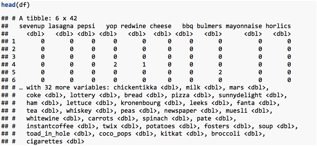
In the data set, all we have is 42 attributes (grocery items) measured on 2000 customers. There is no response variable. Hence, the usual procedures of building a model that explains/predicts the response variable based on the values of the input attributes is ruled out. The class of algorithms that analyzes this type of unlabeled data is called unsupervised learning. The objective of unsupervised learning is to discover hidden patterns in the data. Clustering is an unsupervised learning technique used to uncover distinct clusters of observations within a set of data. Clusters are groups of data-points such that members of the same group have similar features while members of different groups have dissimilar features. At the start of the analysis we do not know how many clusters are there, or if any exist. In clustering technique, the similarity/ dissimilarity between observations or clusters is measured in terms of distance between them.
There are different methods for measuring the distance between observations such as euclidean, manhattan, minkowski etc. Which distance measure to choose will depend on the type of data and the nature of question that is being asked. Euclidean distance is the most common distance measure. It measures the straight-line distance between the data points. In this project, we choose the Euclidean method to measure the distance. Once the distance method is selected, the next question is- how do we measure the distance between two groups of observations, or between a group and a single observation? One method is to compute all pairwise distances between observations in the two clusters and use the average of them.
The K-means clustering algorithm is the most common and computationally efficient clustering technique available. It works with continues variables. However, the disadvantage is that we have to specify in advance the number of clusters to be created.
The objective of K-means clustering is to partition the data {1,2,.,n} into k-clusters {C1, C2,..,Ck} such that:
1. C1 ⋃ C2 ⋃ … ⋃ Ck = {1,2,..,n}
2. Ck ∩ C(k') = 0 for all k≠k'
3. Within-cluster variation is minimum
The following steps summarizes the k-means clustering algorithm:
1. Specify the number of clusters (k) to be created.
2. Select randomly k objects from the data-set as the initial cluster centroids.
3. Re-assign each observation to the cluster whose centroid is closest to that observation (defined using Euclidean distance).
4. For each of the K clusters, update the cluster centroid (the vector of the p feature means for the observations in that cluster).
5. Repeat the last two steps until there is only minimal improvement in the minimization function of total within sum of squares.
The analysis is carried out using R software, in the following steps.
1. Reading the dataset:
As the data file is in excel format, it is opened and read using the read_excel function present in the readxl library.

Thus, a data frame variable df is created.
2. Data exploration / preprocessing:
Missing, invalid and inconsistent values are addressed in this step. Finally, the data is formatted to make it suitable for subsequent analysis. This is a vital step in the analysis process and perhaps consumes the major share of time.
Missing values: The function complete.cases() returns a logical vector indicating which cases are complete. !complete.cases() function is used to obtain the incomplete cases.
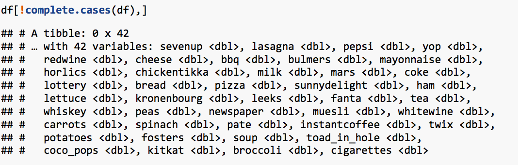 It shows that the data has no missing values.
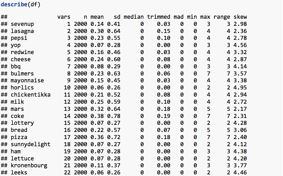
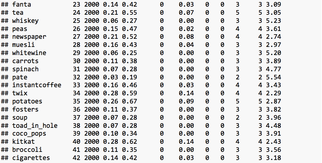
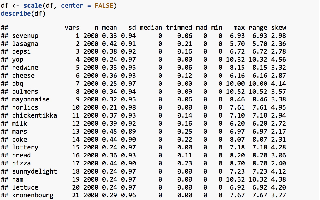
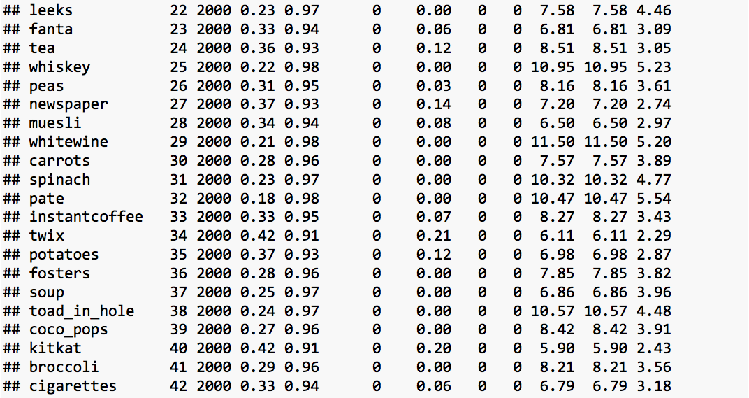
The summary statistics of the imported data is obtained using describe function present in psych library.
Standardization: The value of distance-measures are intimately related to the scale on which the measurements are made. Hence, the data is scaled to avert possible misleading calculations.
3. Finding optimal number of clusters:
A disadvantage of k-means clustering is that we need to specify in advance how many clusters we want the algorithm to “discover”. Fortunately, there are in-built functions to help us estimate the optimal number of clusters for the data-set. One of them is the Elbow or WSS (Within-cluster Sum of Square) method. The WSS method looks at the total within-cluster sum of squares as a function of number of clusters. This function is present in the factoextra package of R.
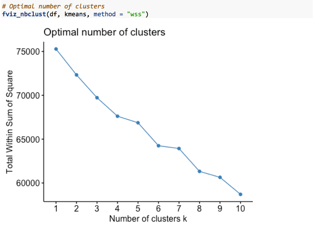 The plot shows that the within-cluster sum of squares decreases with increase in umber of clusters. Due to other practical reasons, we chose to divide the customers into 6 clusters.
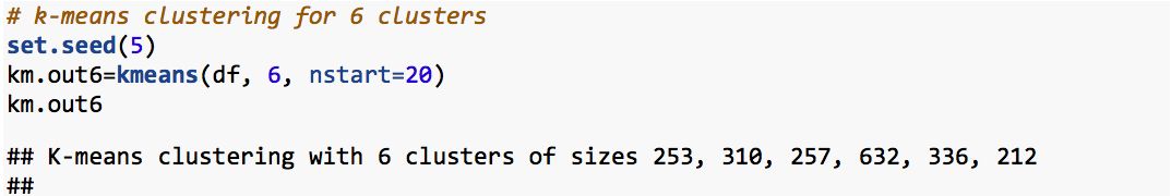
4. K-means clustering:
k-means clustering is performed to segment the cutomers into 6 clusters based on the similarity of items purchased by them. For this, we use the kmeans function present in stats package of R. The output of kmeans function gives the size of each cluster, cluster means, distance between cluster means along with other components.
Before looking into the output of kmeans function, it would be good to check the cluster plot. This is obtained using fviz_cluster function present in the factoextra package of R. Observations are represented by points in the plot, using two principal components that explains the maximum variation in the data.
Plot of clusters:

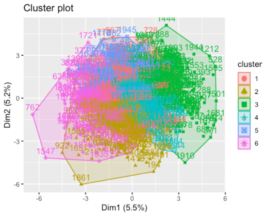
The plot shows that there is considerable overlap between the clusters. Cluster-2 and cluster-5 seems to be the farthest from each other.
Size of clusters:
The size of clusters is given by the size component of kmeans output.
The output shows that:
- Cluster 1 has 635 customers
- Cluster 2 has 259 customers
- Cluster 3 has 251 customers
- Cluster 4 has 304 customers
- Cluster 5 has 209 customers
- Cluster 6 has 342 customers
Cluster means:
The cluster means output shows the value contributed by each attribute to different cluster centroids. The attribues that contribute signiifcantly to each of the cluster centroids are identified in table below:
| Cluster-1 | Cluster-2 | Cluster-3 | Cluster-4 | Cluster-5 | Cluster-6 |
|---|---|---|---|---|---|
| redwine | cheese | milk | leeks | lasagna | |
| bulmers | mayonnaise | tea | peas | chicken-tikka | |
| kronenbourg | bread | muesli | carrots | pizza | |
| whiskey | ham | instant coffee | spinach | ||
| fosters | lettuce | coco pops | potatoes | ||
| broccoli |
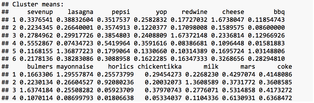
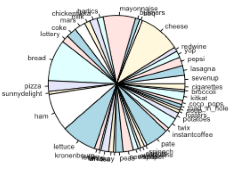
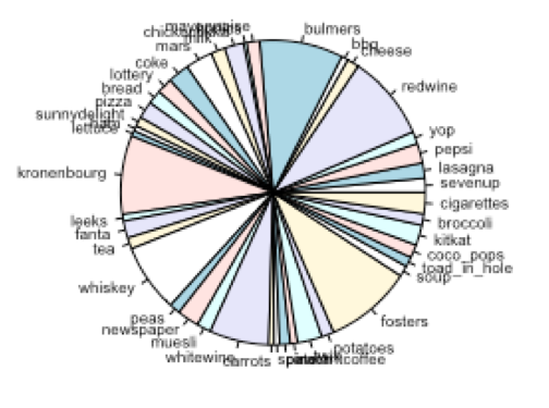
Pie charts: Pie charts showing composition of each cluster is given below:
Cluster-1:
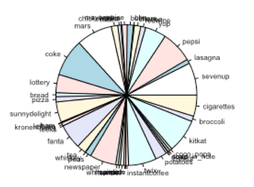
Cluster-2:
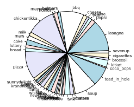
Cluster-3:
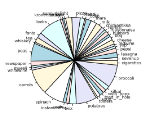
Cluster-4:
Cluster-5:
Cluster-6:
From the compostion of clusters and the significant attributes contributing to clsuter centroids, it can be inferred that:
- Cluster-1 represent the general customers who do not exhibit any strong preferences. But a closer look shows that they tend to buy more soft-drinks and chocolates.
- Cluster-2 represent the customers who prefer alcoholic beverages
- Cluster-3 represent the customers who prefer to prepare sandwiches at home
- Cluster-4 represent the customers who prefer milk/coffee and breakfast cereals.
- Cluster-5 represent the customer group who prefer vegetables
- Cluster-6 represent the customers who prefer fast-food like pizza, lasagna
Distance between cluster centers:
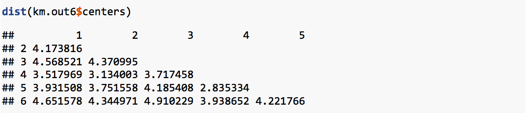
The distance between cluster centers shows that:
- Cluster-1 (general customers) and Cluster-6 (customers who prefer fast-food) are the nearest. It indicates that the general customers and customers who prefer fast-food have similar preferences.
- Cluster-2 (customers who prefer alcoholic beverages) and Cluster-5 (customers who prefer vegetables) are farthest, indicating that they have very dissimilar preferences.
4. Conclusion:
From the analysis presented baove, it can be concluded that the customers of the grocery store are mainly of 6 groups: Group-1: those who prefer to puchase alcoholic beverages Group-2: those who prefer purchase items to prepare sandwiches Group-3: those who purchase breakfast items Group-4: those who purchase vegetables Group-5: those who purchase fast-food Group-6: those who prefer softdrinks
Those who prefer to puchase vegetables have very dissimlar preferences compared to those who prefer alcoholic beverages. Those who prefer softdrinks have similarities to all other groups.
References:
- Image: https://www.itagroup.com/insights/keys-successful-customer-segmentation-cmb-insights